Abstract

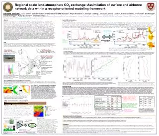
1. Regional scale land-atmosphere CO2 exchange: Assimilation of surface and airborne network data within a receptor-oriented modeling framework Daniel M.Matross1*, Scot Miller2, Steven Wofsy2, Pathmathevan Mahadevan2, Arlyn Andrews3, Christoph Gerbig4, John Lin5, Bruce Daube2, Elaine Gottlieb2, VY Chow2, Bill Munger2, David Hollinger6, Pieter Beckman7, Allen Goldstein1{1Department of Environmental Science, Policy, and Management, University of California Berkeley, 2Harvard University, 3NOAA ESRL GMD, 4MPI Jena, 5University of Waterloo, 6USDA Forest Service, 7UNH Airmap Program} *151 Hilgard Hall, Berkeley, CA 94720 dmatross@nature.berkeley.edu http://nature.berkeley.edu/~dmatross Abstract We quantify and characterize terrestrial CO2 exchange at the regional (~104 km2) scale in the Northeast U. S. and southern Quebec during summer 2004 through an end-to-end model data fusion study. Our dataset is both spatially and temporally representative of the region, consisting of continuous surface concentration data from the NOAA GMD ESRL Argyle Tall Tower and four other concentration monitoring locations throughout the region, and 200 hours of airborne concentration data from the COBRA-Maine airborne campaign. Surface fluxes are characterized by optimizing the parameters of the Vegetation Photosynthesis and Respiration Model (VPRM), a simple biosphere model that integrates satellite data, AmeriFlux eddy covariance measurements, and meteorological fields. The surface flux model is coupled to a Lagrangian atmospheric adjoint model, the Stochastic Time-Inverted Lagrangian Transport Model (STILT), that links point observations to upwind sources with high spatio-temporal resolution. Forward model calculations represent remarkably realistic a priori conditions for Bayesian inversion of the atmospheric concentration data. There is a high amount of redundancy due to spatial and temporal correlation of these observations, which drastically reduces the degrees of freedom in the optimization, emphasizing the need for large amounts of diverse and independent data to constrain even a limited number of parameters. The spatial coverage of airborne data proved strongly complementary with the temporal coverage provided continuous tower observations. The atmospheric concentration dataset provides significant constraint for the model and optimization leads to surface flux parameters with greatly reduced uncertainty. However, the ability to model observed atmospheric CO2 is still limited by errors in the model unrelated to the surface flux parameters: especially atmospheric transport, boundary conditions for the region, and environmental drivers for surface fluxes (e.g. radiation). These errors can be systematic and biased, and since they are unrelated to the surface flux model may lead to biased flux parameters and/or underestimates of parameter uncertainty. Comparisons of forward CO simulations at Argyle and simulations from WLEF, a mid-continental tall tower, demonstrate that transport models are especially prone to error in the Northeast US, especially when weather is dominated by complex, coastal influenced circulations. Forward Model Calculations 1. Carbon Monoxide (CO) Why CO? Forward model runs with CO provide a ready test of the driving meteorology and upstream boundary condition. Since CO does not have major biological sources and sinks, we take the only sources to be fossil fuel emissions (see Gerbig et al., 2003) and biomass burning emissions, calculated from a new biomass burning emission inventory (Wiedinmyer et al., 2006). The fossil fuel inventory is reasonable, so large deviations of model concentrations from measured values are indicative of errors in the winds of underlying meteorological driver for STILT. Errors in transport cannot be optimized through the Bayesian inversion for surface flux parameters. The optimization of surface flux parameters will alias any systematic errors in transport. The differences between a site dominated by continental weather patterns (WLEF) and a site influenced by coastal weather patterns (Argyle) show 1) Transport errors in the underlying STILT driver fields can significantly impact the accuracy of the model 2) Because atmospheric models have difficulty with certain meteorological situations (e.g. coastal transport in the Gulf of Maine), the model will perform more poorly in regions where such transport situations regularly occur. Additionally, forward runs with CO highlight the importance of an accurate boundary condition and including a biomass burning inventory. Inversion for surface flux parameters in CO2 will give no constraint on such errors. Sample integrated footprint functions (log colorscale) Boundary condition incorrect; higher CO than observations Same model, but different regional meteorological regimes { Critical contribution of Canadian fires captured Continental Coastal Data Our dataset is comprehensive and fully representative of the northeast U.S. and southern Quebec for May-September 2004. Components include 1) 200-hours of in-situ airborne observations from the COBRA-Maine aircraft campaign {http://www.deas.harvard.edu/cobra/}, 2) Continuous tall tower observations from the NOAA ESRL GMD Argyle tall tower in central Maine, hourly averaged, 3) Surface concentration data from selected eddy covariance sites, air quality monitoring locations, and temporary sampling locations, hourly averaged Impressive correlation! Figure 5 – Forward STILT + Fossil Fuel Inventory + Biomass Burning inventory calculations (red) of CO (ppb) at WLEF (Park Falls, WI) in August 2004 compared with observations (black). The inset shows contribution of biomass burning CO to the total model signal. Figure 6 – Same as (5), but for Argyle (Argyle, ME). Panels along the side show three sample time-space integrated surface influence function. The top depicting a situation of outflow near along the Eastern seaboard well captured by the model. The center showing where the model transport suggests influence from cities along the St. Lawrence River that is not seen in the observations. The bottom panel depicts a coastal weather pattern the transport drivers handle poorly. Airborne Data Tall Tower Data Argyle Tall Tower (107 m) NOAA ESRL GMD [CO2, CO] 2. Carbon Dioxide (CO2) Forward STILT+VPRM calculations at Argyle tall tower (Figure 7) are able to capture synoptic scale and seasonal variability, but are affected by similar issues as the CO-analyses, namely poorly handled transport by the underlying meteorological drivers and errors in the boundary condition—problems particularly prominent in the northeast U.S. Vertical analysis of the COBRA-Maine airborne data (Figure 8) also suggests that STILT+VPRM hasn’t properly parameterized the rectifier effect, another difficulty stemming from the underlying meteorological driver fields. A similar analysis of CO shows that the model reasonably captures the vertical structure of the measurements, but has a systematic bias in the boundary condition. COBRA-Maine Airborne Campaign {Summer 2004} [CO2, CO, O3] Surface Tower Data Howland Forest (29 m) USDA Forest Service [CO2, CO] Chebogue Point (10 m) UC Berkeley [CO2, CO] {Summer 2004 Only} Figure 1a – University of Wyoming King Air, the airborne platform for COBRA-Maine Thompson Farm (15 m) UNH Airmap [CO2, CO] Harvard Forest (30 m) Harvard University [CO2, CO] Figure 1c – Map of COBRA-Maine flight tracks and surface monitoring locations. Flight tracks are in gray—Bangor Maine (blue square) was the aircraft base. Nearly every flight included fly-bys of Argyle (red triangle) and Howland forest (green circle near Argyle). Figure 1b –3-D flight track of a typical COBRA-Maine flight (11-June-2004; flight 1), demonstrating emphasis on vertical sampling. Coloring follows time of flight. STILT+VPRM Receptor Oriented Modeling Framework We utilize the receptor oriented modeling framework, as described in Gerbig et al., (2003) and Matross et al., (2006) and illustrated below. The major components are an adjoint transport model, STILT, and a surface flux model, VPRM. A fossil fuel inventory and boundary condition complete the accounting. Figure 8 – Vertical averages from COBRA-Maine airborne observations and corresponding forward model results. There are 965 total observations split into 8 x 250m altitude bins. CO results show that the model reasonably captures variation with altitude, but the boundary condition is systematically biased low. CO2 results suggest the model is not properly simulating the covariance between diurnal fluxes and the growth/decay of the boundary layer. Figure 7 – Timeseries (a) of STILT+VPRM calculated mixing ratios (red) and observations (black) of CO2 at Argyle tall tower. Deviations of the model from observations can be explained by any of the issues suggested by CO modeling—boundary condition, transport errors—or VPRM surface flux parameters in need of adjustment. Bayesian inversion can only address the latter. A comparison of afternoon average values measure vs. modeled is shown in (b). Assimilated Meteorology Particle locations Surface inlfluence “footprint” STILT – Stochastic Time-Inverted Lagrangian Transport Model STILT (Lin et al., 2003) is analogous to the adjoint of an Eulerian transport model, designed to calculate footprints representing the sensitivity of the mixing ratio at a receptor location to a given upstream surface flux. We utilize the 45-km Brazillian-version Regional Atmospheric Modeling System (BRAMS) as our primary meteorological driver. Assimilated winds (a) drive a set of particles, which represent air parcels, backwards in time from a location and time designed to coincide with a measurement (the “receptor”, e.g. Argyle tower) (b). A surface influence function (c), the “footprint”, can be calculated from the particle locations. This footprint is defined as the influence of upstream surface sources on the composition of air at a particular measurement point. It links the measurement to the upstream surface fluxes with high spatio-temporal resolution. Inversion Results Although the VPRM calculates gross ecosystem exchange (GEE) and respiration (R), there is strong correlation between these two parameters—rendering separate inversion parameters on GEE and R difficult to constrain. Atmospheric data can provide a much tighter constraint on their sum (NEE). However, when photosynthesis and respiration are nearly balanced, NEE will be near zero, which introduces instability in a multiplicative optimization factor. These dual limitations lead us to use an additive parameter (dk) in a Bayesian inversion of the network atmospheric data. Thus, modeled mixing ratio at the receptor point is defined by Equation 1, where k indexes all vegetation classes, with dkprior = 0 for all vegetation classes. The parameter results are shown in Figure 9. We have achieved a successful Bayesian inversion for our additive surface flux optimization parameter using all the available data, greatly reducing the uncertainty. Table 1 demonstrates the constraints placed by various data combinations, using a formally calculated (Rodgers, 2000) measure of “degrees of freedom”. The total number of degrees of freedom equals the total number of parameters in the inversion (in this case 11, one additive parameter for each vegetation class) and is split between degrees of freedom with information leading to parameter constraint (DF signal) and those related entirely to noise (DFnoise). More degrees of freedom for the signal indicated higher constraint. One conclusion that can be drawn from Table 1 is that airborne data and tower data are strongly complimentary, because airborne data provides broad spatial coverage and tower data provides broad temporal coverage. Table 2 gives an example of the application of inversion results to calculations of NEE in the Northeast U.S. and southern Quebec. (b) (c) (a) Figure 2—STILT calculations. Assimilated wind fields (a) drive particles representing air parcels, which are transported backward in time (b) from a receptor point. Particle locations are used to calculate a surface influence function, the time-space integral of which is visualized in (c). Marginal cost of constraint is high! One tower gives lots of constraint, but a second one provides an order of magnitude less additional constraint. Information within multiple towers is redundant. Eq. 1 Figure 9—Prior and posterior parameter values, along with associated estimates of uncertainty, using all network data. This is indicative of a successful Bayesian inversion. VPRM – Vegetation Photosynthesis and Respiration Model • Initial Parameters Fit to Ameriflux eddy covariance data GEE= λ (Tscalar Wscalar  Phscalar )EVI1 /(1+ SW/SW0) x SW • National Land Data Assimilation System (NLDAS) inputs Airborne data and tower data are strongly complementary. A surface network and a single tower + airplane supply similar constraint. Towers give temporal coverage, aircraft give spatial coverage R = α Tair + β • MODIS-derived Inputs VPRM (Pathmathevan et al.,2007) is a data-driven diagnostic biosphere flux model. Satellite data provide independent information on the spatial and phenological variations of gross primary production using the Enhanced Vegetation Index (EVI) and Land Surface Water Index (LSWI), both from MODIS-Terra. Model parameters {3 parameters x 11 vegetation classes = 33 total paramters, time invariant} are initially determined through fitting to eddy covariance data from AmeriFlux sites. The model uses temperature and incident solar radiation from retrievals based on data from the North American Land Data Assimilation System (Mitchell, et al., 2003). VPRM calculates net ecosystem exchange (NEE) of CO2 for each of 12 vegetation classes in each grid square separately, scaled by vegetation fraction. Figure 3—VPRM vegetation classes in the northeast US and southern Quebec Table 2—VPRM-calculated NEE [tons/ha] for the northeast U.S. and southern Quebec (41-52˚N, 67-80˚W) for each month in summer 2004 based on added optimization factors calculated through Bayesian inversion of all network data. Maximal constraint requires surprisingly large number of observations Table 1—Constraint placed on the Bayesian Inversion by various combinations of data, as measured by degrees of freedom (DF). Total DF equals the number of parameters and are split between those contributing information (signal) about the data and those contributing no information (noise). A higher signal value indicates the data places more constraint on the parameters in the inversion. N refers to afternoon hours of tower data or sub-sampled 20-second averages of airborne data. • Conclusions & Take-Home Messages • Transport errors in underlying meteorological fields, errors in environmental driver fields (e.g. radiation), and incorrect boundary conditions lead directly to errors in model calculated mixing ratios of trace gases • Assimilation of atmospheric data through Bayesian inversion to optimize surface flux parameters will not reduce these errors, although overall parameter uncertainty may be significantly reduced, a traditional metric of a successful inversion • It takes a large amount of atmospheric data to constrain even a limited number of parameters; multiple observations will have redundant information about surface fluxes • Airborne and tall tower data are strongly complimentary for inversion studies, airborne data provides broad spatial coverage and tall tower data broad temporal coverage Meteorological Product Figure 4—Model –data fusion schematic Model-Data Fusion VPRM fluxes and a fossil fuel inventory are convolved with STILT-calculated surface influence functions {particles are always run backward in time}, then added to regional boundary condition to complete the “forward” model run for an set of receptor points. The “inverse” model applies atmospheric data in a Bayesian framework (Rodgers, 2000) to optimize an additive parameter (dk; k indexes vegetation class, a priori value is 0) to the VPRM fluxes. An additive parameter is needed because of the high correlation of GEE and R with each other, and the potential for instability in a multiplicative parameter when photosynthesis and respiration are in balance. Careful accounting of the error covariance is outlined in Matross et al., (2006). Tracer boundary condition Fossil fuel inventory STILT Environmental Drivers “Forward Model” Model Concentrations References Gerbig, C., J. C. Lin, S. C. Wofsy, B. C. Daube, A. E. Andrews, A. E., B. B. Stephens, P. S. Bakwin, and C. A. Grainger (2003). Towards constraining regional scale fluxes of CO2 with atmospheric observations over a continent: 2. Analysis of COBRA data using a receptor oriented framework. J. Geophys. Res., 108, D4757, 10.1029/2003JD003770. Lin, J. C., C. Gerbig, S. C. Wofsy, A. E. Andrews, B. C. Daube, K. J. Davis, C. A. Grainger, The Stochastic Time-Inverted Lagrangian Transport Model (STILT): Quantitative analysis of surface sources from atmospheric concentration data using particle ensembles in a turbulent atmosphere (2003). J. Geophys. Res., 108, D4493, 10.1029/2002JD003161. Matross, D. M., A. Andrews. M. Pathmathevan, C. Gerbig, J. C. Lin, S.C. Wofsy, B. C. Daube, E. W. Gottlieb, V. Y. Chow, J. T. Lee, C. Zhao, P .S. Bakwin, J. W. Munger, and D. Y. Hollinger (2006). Estimating regional carbon exchange in New England and Quebec by combining atmospheric, ground-based and satellite data, Tellus, 58B, 344-358. Mitchell, K. E., D. Lohmann, P. R. Houser, E. F. Wood, J. C. Schaake, A. Robock, B. A.Cosgrove, J. Sheffield, Q. Duan, L. Luo, R. W. Higgins, R. T. Pinker, J. D. Tarpley, D. P. Lettenmaier, C. H. Marshall, J. K. Entin, M. Pan., W. Shi, V. Koren, J. Meng, B. H. Ramsay, and A. A. Bailey (2004). The multi-institution North American Land Data Assimilation System (NLDAS): Utilizing multiple GCIP products and partners in a continental distributed hydrological modeling system. J. Geophys. Res., 109, D07S90, doi:10.1029/2003JD003823. Pathmathevan, M., S. C. Wofsy, D. M. Matross, X. Xiao, A. L. Dunn, J. C. Lin, C. Gerbig, J. W. Munger, V. Y. Chow, and E. Gottlieb (2007). A satellite-based biosphere parameterization for net ecosystem CO2 exchange: Vegetation photosynthesis and respiration model (VPRM). Global Biogeochemical Cycles, in press. Rodgers, C. D. (2000), Inverse Methods for Atmospheric Sounding: Theory and Practice, 238 pp., World Sci., River Edge, N. J. Wieinmyer, C., B. Quayle, C. Geron, A. Belote, D. McKenzi, X. Y. Zhang, S. O’Neill, and K. K Wynne (2006). Estimating emissions from fires in North America for air quality modeling, Atmospheric Environment., 40 (19), 3419-3432. Influence function Vegetation Fluxes [NEE] Optimization {aka “Inverse Model”} Adjustable Parameters λ, α, dk VPRM Atmospheric Data