Download
1 / 32

E N D
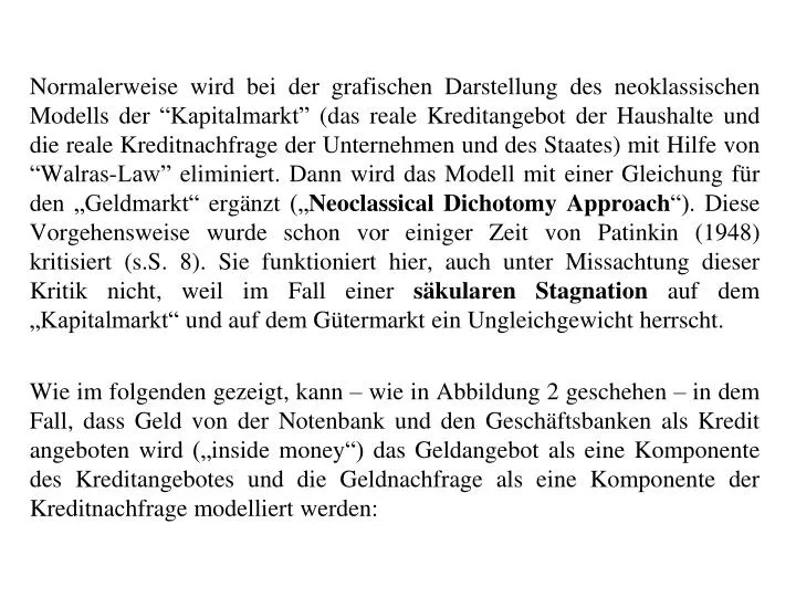
Normalerweise wird bei der grafischen Darstellung des neoklassischen Modells der “Kapitalmarkt” (das reale Kreditangebot der Haushalte und die reale Kreditnachfrage der Unternehmen und des Staates) mit Hilfe von “Walras-Law” eliminiert. Dann wird das Modell mit einer Gleichung für den „Geldmarkt“ ergänzt („NeoclassicalDichotomy Approach“). Diese Vorgehensweise wurde schon vor einiger Zeit von Patinkin (1948) kritisiert (s.S. 8). Sie funktioniert hier, auch unter Missachtung dieser Kritik nicht, weil im Fall einer säkularen Stagnation auf dem „Kapitalmarkt“ und auf dem Gütermarkt ein Ungleichgewicht herrscht. Wie im folgenden gezeigt, kann – wie in Abbildung 2 geschehen – in dem Fall, dass Geld von der Notenbank und den Geschäftsbanken als Kredit angeboten wird („insidemoney“) das Geldangebot als eine Komponente des Kreditangebotes und die Geldnachfrage als eine Komponente der Kreditnachfrage modelliert werden:
Overview 1. The Problem of Walras 2. The Neoclassical Dichotomy Approach & Patinkin’s Criticism 3. Patinkin’s Solution: A Real Wealth Effect 4. Weil’s Criticism: Money Is Not Net Wealth in Ricardian Economies 5. Institutionally Correct Modelling of Money Supply 6.1. Example: A Textbook Macromodel 6.2. Example: The Case with N Goods 6. Conclusions 7. Appendix: The Inconsistency of the Neoclassical Dichotomy 8. Literature Detailed Paper “Walras' Law and the Problem of Money Price Determinacy“ available at: http://ssrn.com/abstract=1258939
1. The Problem of Walras • Since Walras (1874) has shown that the validity of the budget constraints implies an equilibrium on the nth market, if n-1 markets are in equilibrium, there is one equation missingto unambiguously determine the money prices of goods. • Some researchers have therefore given up the idea that money prices are well determined: • In his book “Interest and Prices” Woodford (2003, p. 34) cites Wicksell (1898, pp. 100-101), “who compares relative prices to a pendulum that always returns to the same equilibrium position when perturbed, while the money prices of goods in general are compared to a cylinder resting on a horizontal plane, which can remain equally well in any location on the plane to which it may happen to be moved”. • Contrary to this view, I show in the following: If money supply is modelledin an institutionally correctway, there will always be “an equation left” to allow for money price determinacy: Hence money prices too have the properties of a pendulum.
1. The Problem of Walras • In an economy with N goods markets, only N-1 prices can be determined: • Household budget with N goods: • Adding up the budgets of all H households: • Rearranging the sums: ≡ Lange (1942, p.50):“Walras’ Law”
1. The Problem of Walras • Therefore, if N-1 markets are in equilibrium: • The Nth market too must be in equilibrium, as a subtraction of (2) from (1) shows: ≡ Patinkin (1965, p.35) :“Walras’ Law”
1. The Problem of Walras • Consequently, if all households keep their budgets, only N-1 independent equations exist. => Even if the “counting criterion” holds, => it is only possible to determine N-1 relative prices in terms of the numéraire. The price of the numéraire is set equal to 1. • Solution following the “Neoclassical Dichotomy Approach”: • To determine the N money prices of all goods we can simply “add a money market equation” to determine the money price of the numéraire: “If the equation system is linear and the coefficient matrix of the linear equations is non-singular, the equality of the number of equations and the number of unknowns is sufficient for the existence of a unique solution.” N-1 relative prices determined by the N-1 independent market equilibrium conditions “Money price” of the numéraire
2. The Neoclassical Dichotomy Approach & Patinkin’s Criticism • Patinkin’s criticism of the “Neoclassical Dichotomy Approach”: • It leads to a logical contradiction: • If there is a general market equilibrium on all N markets plus the money market, • a duplication λ = 2of all money prices will leave the N goods markets in equilibrium, since it does not change the relative prices: • The money market equation however will display excess demand: • However, by Walras’ Lawthis is not possible, since the money market must be in equilibrium, if all other markets are in equilibrium. • Therefore, following Patinkin, the Neoclassical Dichotomy Approach leads to a logical contradiction!
3. Patinkin’s Solution: A Real Wealth Effect • Patinkin’s solution: The Real-Balance-Effect • Patinkin (1949) proposed the introduction of a wealth-effect by adding the real value of money holdings as a positively valued argument in the demand functions for goods: • such that an increase of the price level leads to a decrease of the real value of money wealth and hence the emergence of excess supply of goods, • which by Walras’ Law is consistent with excess demand for money:
4. Weil’s Criticism: Money Is No Net Wealth • Weil (1991) criticism: Money is no net wealth! • Following Barro’s “Ricardian Equivalence” Weil shows that in a standard Ricardian (infinitely-lived representative agent) economy, even outside money holdings cannot be net wealth. • The basic argument for the simplified case of a constant interest rate i = it and an infinite time horizon, t = 1,2,.. ∞: Present value of the opportunity costs of holding money Value of money holdings
4. Weil’s Criticism: Money Is No Net Wealth • Weil (1991) criticism: Money is no net wealth! • Mathematically equivalent alternative statement of the argument: • Barro’s (1974) proof that government bonds are no net wealth under such circumstances: If the government increases its consumption and finances this by issuing government bonds, the representative household receives, on one hand, additional interest payments from these bonds plus the face value at the end of maturity. On the other hand, the present value of these payments equals exactly the additional future taxes, which the household has to pay to finance these interest payments plus redemption. Consequently the net present value of holding these bonds is zero for the household. • Analogously, if the government increases its consumption and finances this by paying with banknotes, the representative household does, on one hand, not have to pay additional future taxes to finance any interest payments or the redemption, but receives, on the other hand, no interest payments and no repayment of the face value from holding these banknotes. Consequently the net present value of holding these banknotes in a Ricardian economy is for the same reasons zero as the net present value of holding government bonds. If instead of government consumption lump sum transfers to households are assumed, the argument does not change. The only difference in this case is that the disposable income of households stays constant at the end of the day, while in the case of government consumption, the disposable income is reduced.
5.1. Institutionally Correct Modelling of Money Supply: A Textbook Macromodel • The following calculations show based on the standard three market textbook macromodel that • ifmoney supply and demand is modeled • in a realistic, institutionally correct way, there is always an equation left, which can be used to determine the money prices of goods – even in an Ricardian economy, where money is no net wealth.
5.1. Institutionally Correct Modelling of Money Supply: A Textbook Macromodel
5.1. Institutionally Correct Modelling of Money Supply: A Textbook Macromodel There will not necessarily be an equi-librium on the goods market: There will not necessarily be an equi-librium on the goods market:
6. Alternative Solution: Institutionally Correct Modelling of Money Supply: A Textbook Macromodel There will not necessarily be an equi-librium on the goods market: There will not necessarily be an equi-librium on the goods market:
5.1. Institutionally Correct Modelling of Money Supply: A Textbook Macromodel
5.1. Institutionally Correct Modelling of Money Supply: A Textbook Macromodel
5.1. Institutionally Correct Modelling of Money Supply: A Textbook Macromodel
5.1. Institutionally Correct Modelling of Money Supply: A Textbook Macromodel Only if money demand equals money supply, the goods market is in equilibrium!
5.1. Institutionally Correct Modelling of Money Supply: A Textbook Macromodel
5.1. Institutionally Correct Modelling of Money Supply: A Textbook Macromodel • If money supply is larger than money demand, there will be excess demand for goods, which will cause the price level for goods to increase: • If real money demand depends (as usual) on the real transaction volume divided by the money velocity, this increase of the price level will cause real demand supply to decrease so that the excess supply of money and – simultaneously – the excess demand for goods disappears: < = = >
5.1. Institutionally Correct Modelling of Money Supply: A Textbook Macromodel Digression: Consequently, if money supply is institutionally correctly modelled, the above three market macromodel can be easily transformed into the standard textbook form: If the assumption is made that the budget constraints hold, three market equilibrium conditions are sufficient to guarantee a general market equilibrium: Either Labor market equilibrium: Capital market equilibrium: Money market equilibrium: Or Labor market equilibrium: Goods market equilibrium: Money market equilibrium: Consequently, the standard textbook system of market equilibrium conditions is compatible with the above described “outside money” case, as well as with the “inside money” case. The standard textbook model has in fact two monetary interpretations. The same holds of course for the Keynesian fixed price version of this model. => Goods market equilibrium => Capital market equilibrium
5.1. Institutionally Correct Modelling of Money Supply: A Textbook Macromodel • As this text book macromodel shows, if money supply differs from money demand, a “transaction volume effect” will cause the price level to adjust and restore an equilibrium on the goods market. • Consequently it is a “transaction volume effect” the determines the price level – there is no need for Patinkin’s “wealth effect” (or “real balance effect” or “Pigou effect”). • The following calculations show that the same holds of course for the case of an economy with N goods and H households:
5.2. Institutionally Correct Modelling of Money Supply: The Case with N Goods • Starting point: An economy with H households, N goods markets and money supplied by the government: • Household budget with N goods plus money demand: • Government budget with N goods plus money supply: • Adding up the budgets of all H households and the government:
5.2. Institutionally Correct Modelling of Money Supply: The Case with N Goods • IfN-1 markets for goods are in equilibrium: • The Nth market will not necessarily be in equilibrium, as subtracting of (4) from (3) shows: • Consequently, to make sure that the Nth goods market is in equilibrium, it is necessary to assume that the budget constraintshold, the N-1 markets are in equilibriumand that money demand is equal to money supply!
5.2. Institutionally Correct Modelling of Money Supply: The Case with N Goods • If money supply is larger than money demand, there will, as equation (3) shows, generally be excess demand for goods: • Following the standard assumption, nominal money demand of a household depends on the nominal transaction volume of the household:
5.2. Institutionally Correct Modelling of Money Supply: The Case with N Goods • Under this assumption, an increase of the price level will cause money demand to grow so that the excess supply of money and – simultaneously – the excess demand for goods disappears: • As this model with N goods and H Households shows, if money supply differs from money demand, it is again a “transaction volume effect”, which will cause the price level to adjust and restore an equilibrium on the goods market. • Consequently here too, it is a “transaction volume effect” the determines the price level – there is no need for Patinkin’s “wealth effect”. < = = >
6. Conclusions • If money supply and money demand is modelled based on a realistic institutional setup in the budget constraints and market equations, the resulting number of independent equations is always equal to the number of goods. • Consequently, if the “counting criterion” holds, there are always enough equations to determine the money prices of all goods in an economy. • If money demand depends on the transaction volume of the economy, it will be a “transaction volume effect”, which restores the monetary equilibrium but not a “wealth effect”. In so far, Patinkin (1948) is wrong and the Neoclassical Dichotomy Approach is right.
6. Conclusions • However, Patinkin (1948) is right and the Neoclassical Dichotomy Approach is wrong in another important point: • Money price determinacy excludes the assumption of “zero degree homogeneity” in money prices of supply and demand functions: A realistic institutional setup of money supply and money demand excludes the assumption of “zero degree homogeneity”. As the following appendix shows, if money supply and demand are modelled in an institutionally correct way, the assumption of “zero degree homogeneity” in money prices, leads to a logical contradiction. • As a result of this all: The standard procedure used in many monetary models, to “eliminate one market by Walras Law” and add a “money market” is correct.
7. Appendix: The Inconsistency of the Neoclassical Dichotomy • Under an institutionally correct setup of money supply, the classical assumption of degree 0 homogeneity in money prices of the demand and supply functions, • leads to a logical contradiction as the following shows: Starting with a general market equilibrium so that following eq. (3):
7. Appendix: The Inconsistency of the Neoclassical Dichotomy • A multiplication of all money prices by a factor λ ≠ 1 yields: • Given the assumption of zero degree homogenty in money prices this equals • what contradicts the assumption that λ ≠ 1. = 0 = MS
8. Literature For a detailed paper with an extension of the argument to a DSGE-Model see: http://ssrn.com/abstract=1258939