Astronomical Information Processing System
AIPS++ is a comprehensive system for processing astronomical data, featuring an extensive set of libraries, toolkits, and applications. Designed by astronomers and programmers, it offers sophisticated features for observatories and data processing.


Astronomical Information Processing System
E N D
Presentation Transcript
Astronomical Information Processing System C++, scripting, GUI’s, libraries, toolkits and applications Designed by a team of astronomers and programmers Developed by an international consortium of observatories Fourth public release (v1.6) available here! http://aips2.nrao.edu
AIPS++ Glish logger Standard Gui viewer
AIPS++ organizational structure • AIPS++ Executive Committee • Butcher (ASTRON), Crutcher (NCSA), Diamond (JBO), Ekers (ATNF), Vanden Bout (NRAO; Chair) • Project Management reports to EC • Kemball (NRAO), McMullin (NRAO) • Site Managers manage local staff, work with PM • Killeen (ATNF), Noble (JBO), Noordam (ASTRON), Plante (NCSA) • AIPS++ User Group advises PM • Balser (NRAO), H. Dickel (UIUC), Fomalont (NRAO), Viallefond (Obs. De Paris), Owen (NRAO), van Langevelde (JIVE), O'Neil (NAIC), Staveley-Smith (ATNF), Oosterloo (ASTRON), Lucas (IRAM), Pauls (Chair, NPOI), Willis (DRAO) • AIPS++ Technical Advisory Group (TAG) will form and meet this year • Local AIPS++ User Groups • NRAO AIPS++ User Group, BIMA User Group, plus others
Facility use of AIPS++ • Green Bank Telescope commissioning and science • Parkes Telescope 21cm multi-beam observations • WSRT TMS on-line system • Joint Institute for VLBI in Europe correlator • Navy Prototype Optical Interferometer development and observing • HIA/DRAO/ACSIS project for post-correlation processing into an image cube • ATNF MOPRA telescope for mm observing (in development) • Consortium data processing and pipelines • Under evaluation by SMA for commissioning and data reduction.
Software engineering practices • Traditional software engineering practices • Requirements documents • Coding rules and standards • Design review • Code review process • Unit testing • Daily automated testing of entire system • Change control process • Quality Assurance Group • Code cop • Chief tester • Robust code management and distribution system • Disciplined 6 month plan-design-implement-test-release process
Operations • C++ • Bulk of code (> 1,700,000 lines) • C++ libraries have wide range of general utilities for data access, display, calibration and imaging. • Connected to IDL-like command language and GUI interface • About 130 person-years effort • ~12,000 lines of code per person per year • Good code productivity
Synthesis development: scientific completeness • Data fillers • available for most consortium instruments and several archive and interchange data formats • Editing and visualization • editing and visualization of visibility data • Calibration • solvers for visibility-plane calibration effects; ability to apply image-plane effects. • Imaging • a range of imaging contexts (mosaic, wide-field etc.) and deconvolution algorithms supported. • Image analysis and visualization • capable image visualization and analysis tools
Basic principles in synthesis design • Scientific access at multiple levels • High-level, integrated synthesis applications, and • A toolkit of low-level synthesis capabilities. • Scientific freedom for end-users • Support custom reduction and data exploration through scripting using the synthesis toolkit. • Toolkit applicable to general interferometry • Instrument independence • Use of a generic data format, as well as calibration and imaging formalism. • New approaches to data reduction • Improved algorithms, support for new instruments (e.g. ALMA) and automated reduction such as pipelines.
Connected-element end-to-end reduction A important element of scientific integration efforts: • NRAO has focused on VLA reduction • Strategy: • Select designated test data in all observing modes • Scientific user groups reduce the data (in collaboration with the project) • Assess usability improvements based on their experience • Inter-compare with other packages • Catalog the reduction scripts and test data in the system • Use in documentation, tutorial examples and automated system testing • Other data also selected by the user groups and processed independently • Similar efforts underway at BIMA, WSRT and ATNF
Structure of applications Multi-level access possible: Guided reduction, integrated tasks Highest level access, non-specialist users, pipeline reduction Custom scientific reduction and scripting Intermediate synthesis tools (imaging, calibration, image analysis) Basic astronomical scripting Lowest level tools (data access, display, computation)
User interface architecture Automated GUI (toolmanager) Custom GUI’s Command-line interface All tools and functions
Tool manager • Automatic GUI to manage / create individual tools • Constructed from meta-information Search for key phrases List of available types of tools, grouped by package and module
Tool manager • Creating an individual tool
Tool manager • Standard parameter entry • Constructed from meta-info • Intelligent data entry • Tied to other tools • e.g. catalog to get files • e.g. viewer to see images • e.g. regionmanager • Cut and Paste • Save/Restore • Commands • Can be viewed and executed • Saved to a script • Executed in batch • Help • Tight connection to appropriate web-based help
Intelligent data entry capabilities • Specialized data entry to simplify retrieval of information
Scripter • Aids construction of Glish scripts • Toolmanager and wizards can write equivalent Glish commands to the scripter – these can then be adapted by users
Tools: general purpose • table: • access to all AIPS++ data • tablebrowser: • edit, plot, query, and select data. Configurable. • viewer: • display images, tables, measurementsets • pgplotter: • plotting of Glish variables using the Caltech PGPLOT library • quanta and measures: • measured quantities with units, coordinates, and reference frames; and their conversion • catalog: • file manager
Tools: tablebrowser • Used to show, edit, select, query tables
Tools: pgplotter • Plots from Glish and C++ • Familiar PGPLOT commands
Tools: Quanta • Values + units: [value=1.905, unit=‘m’] • Many conversions supported
Tools: Measures • Quanta plus coordinates and reference systems • Many conversions supported • Calculate from JPL DE200, DE405; or user-supplied, ephemeredes
Tools: File Catalog • Used to create, edit, view, delete files
Applications • dish: • interactive single dish reduction • msplot: • interactive visibility plotting and editing • calibrater, imager, and simulator: • calibration and imaging using Hamaker, Bregman, Sault generic model • image: • statistics, histograms, moments. • Image display using viewer • image calculator • image regions • image polarization • componentmodels: • modelling of sky by discrete components
Imaging and calibration • Based on Hamaker-Bregman-Sault measurement equation • Allows integration of single dish and synthesis • Extensive development of new formalism for telescope data processing • Many new capabilities both in imaging and calibration • Integrates new deconvolution algorithms • Allows physical models of calibration effects in both antenna and sky planes • e.g. parametrized phase screen across an array • e.g. parametrized band-passes • e.g. non-isoplanatic imaging
Single-dish development • GBT support • Utilities developed in support of GBT commissioning • Pointing/focus, data examination, back-end testing • Data filler expanded to track GBT on-line format • General single-dish reduction • Expansion of dish tool • Closer integration of single-dish and interferometry overall • Significant progress in single-dish imaging • User outreach • Tutorials • Workshop with Arecibo users and reciprocal site visits
Applications: dish NRAO 12m observations of Comet Hale-Bopp, fit with first order polynomial and three component Gaussian fit. Line identifications from JPL catalog (added via AIPS++ plugin)
Single-dish imaging End-to-end single-dish reduction: GBT image of Cygnus Loop at 800MHz processed end-to-end in AIPS++. The original GBT FITS files for this observation are checked into the AIPS++ data repository and the end-to-end reduction may be repeated using the test function imagersdtest()
Synthesis data format • Data format • Visibility data are stored in an AIPS++ table defined as a Measurement Set (MS). • Current revision is v2.0: (Note 229) • Carefully chosen to be compatible with the calibration and imaging formalism (HBS). • Instrument-independent; but can be customized as needed. • VLBI support. • Improved integration of single-dish and synthesis data. • Support for advanced synthesis reduction. • Main table for basic data; sub-tables for auxiliary data.
Data fillers • Data fillers for specific synthesis instruments: • ATCA • WSRT • VLA • BIMA • MERLIN (new MERLIN data format; initial version) • VLBA (initial version) • Data fillers for archive and interchange formats: • UVFITS • FITS-IDI (see VLBA) • FITS binary table archive format for MS • Other converters (e.g. SCN etc)
Data access, display and editing • Data access and summary • using ms tool. • Visibility visualization and editing: • using msplot tool • utility display methods in imager and calibrater • transfer of display and editing capabilities to Display Library underway • Editing • command-based and automated editiing • available in flagger and ms tool • new automated editing tool (autoflag) • Concatenation • using msconcat tool. • Does physical concatenation. • Currently requires constant data shape throughout the MS, as defined by the number of polarization correlations (e.g. XX, XY) and the number of frequency channels. • Merges all main table data, and all required sub-tables.
Applications: msplot • Interactive visibility plotting and editing Many different types of plot • e.g. Iterate over antennas for diagnosis of problems • e.g. Iterate over fields for mosaic observations
Applications: msplot • Can edit on any single plot Regions to be flagged
Applications: msplot Real vs imaginary of Visibility Amplitude vs phase Flagging regions
Applications: msplot • Image-like display and editing • Uses standard viewer tool • Axes can be: • Interferometer • Time • Channel • Polarization • Show and edit in any order
Automated editing • Vital for automated pipeline reduction • Heuristics supported: • UV-plane binning (as left) • Median clip in time and frequency • Spectral rejection (spectral line baseline fitting) • Absolute clipping in a clip range Calibrator 0234+285, VLBA project BK31 (Kemball et al.)
Visibility-plane calibration • Visibility-plane components supported in calibrater • P - parallactic angle correction (pre-computed). • C - polarization configuration (pre-computed). • G - electronic gain, solvable. • T - atmospheric correction, solvable. • D - instrumental polarization response, solvable. • B - bandpass response, solvable. • F - ionospheric correction, pre-computed from global, empirical model (PIM) (initial version). • Pre-computed, or solved using chi-squared computed from the Measurement Equation (ME). • Pre-averaging, phase-only solutions, and reference antenna selection available in solver.
Image-plane calibration • Image-plane calibration supported in imager • Only pre-computed calibration components supported at present. • Primary beam voltage pattern, including beam squint • Wide range of recognized voltage patterns; configured using a voltage pattern utility (vpmanager). • Image-plane solvers in prototype development (a difficult problem).
Calibration tables • AIPS++ calibration information stored in AIPS++ tables • Format chosen to be compatible with MS and ME. • Supports a range of calibration component types: • Antenna-, or interferometer-based. • Pre-computed or solvable. • Parametrized or discretely sampled. • Image or visibility-plane (image-plane pending solver). • Current revision is v2.0 (see AIPS++ Note 240). • Full access to calibration table data. • Utility for polynomial fitting and re-gridding developed by BIMA group.
Imaging capabilities • Imaging from synthesis and single dish data • Supports polarimetry, spectral-line, multiple fields, mosaicing, non-coplanar baselines (simultaneously) • Also single dish OTF, holography • Clean algorithms: Hogbom, Clark, Schwab-Cotton, Multi-scale • Incremental multi-field deconvolution • Non-Negative Least Squares and Maximum Entropy deconvolution • Supports imaging in a wide range of coordinate systems • Tracks moving objects • Discrete image component processing • Flexible in image size (2n not needed) • Novel “sort-less” visibility gridding algorithm • Advises on argument settings • User can “plug-in” customized (Glish) modules • Pixon deconvolution available in the image plane
End-to-end example: 8 GHz VLA mosaic observation of Orion • Data from Debra Shepherd (NRAO); project DSTST • Filling, editing, calibration and imaging of VLA export tape via a Glish script: # Wait for each result before proceeding dowait:=T # load definitions of synthesis processing functions include ‘synthesis.g’; # fill data include 'vlafiller.g'; ok:=vlafillerfromdisk(filename="N13522.vla" , msname="orion.ms" , project="DSTST" , bandname="X"); # flag known bad data myflagger:=flagger(msfile="orion.ms" ); ok:=myflagger.quack(scaninterval="5.1s" , delta=‘10.0s’, trial=F); ok:=myflagger.setantennas(ants=21); ok:=myflagger.timerange(starttime="21-SEP-2000/11:15:48", endtime="21-SEP-2000/13:38:18", trial=F); ok:=myflagger.filter(column="DATA", operation="range", comparison="Amplitude", range='1e-6Jy 1e3Jy', trial=F); myflagger.done();
End-to-end example: Orion calibration and imaging (8 GHz VLA mosaic) # initialize models of known sources myimager:=imager(filename="orion.ms" ); ok:=myimager.setjy(fieldid=1, spwid=-1, fluxdensity=-1.0); ok:=myimager.setjy(fieldid=2, spwid=-1, fluxdensity=-1.0); # calibrate flux scale and visibilities mycalibrater:=calibrater(filename="orion.ms" ); ok:=mycalibrater.setdata(msselect='FIELD_ID in [1,2]'); ok:=mycalibrater.setsolve(type="G" , t=300, table="orion.gcal"); ok:=mycalibrater.solve(); ok:=mycalibrater.fluxscale(tablein='orion.gcal', tableout='orion.ref.gcal', reference='0518+165', transfer='0539-057'); ok:=mycalibrater.setdata(msselect=''); ok:=mycalibrater.setapply(type="G", table="orion.ref.gcal", select="FIELD_NAME=='0539-057'"); ok:=mycalibrater.correct(); mycalibrater.done();
End-to-end example: Orion calibration and imaging (8 GHz VLA mosaic) # make and deconvolve mosaic image ok:=myimager.setimage(nx=300, ny=300, cellx=‘4.0arcsec’, celly=‘4.0arcsec’, stokes=‘I’, spwid=[1, 2]); ok:=myimager.setdata(spwid=[1, 2] , fieldid=3:11 , msselect=''); ok:=myimager.weight(type="briggs" , robust=-1); ok:=myimager.setvp(dovp=T, dosquint=F); ok:=myimager.mem(algorithm="mfentropy", niter=100, sigma=‘4mJy’, displayprogress=T, model="orion.mem"); myimager.done(); • 10 pointing VLA 8 GHz mosaic of Orion processed entirely in AIPS++ • Filled from VLA export tape, edited, calibrated, and imaged, displayed using AIPS++ tools
Continuum calibration and single-field imaging • Project AP366: • Patnaik, Kemball et. al. • 24-hour VLA observation in A-configuration of a sample of gravitational lenses • Continuum imaging of 0957+561 at 5 GHz shown here • Phase calibrator 0917+624. • Amplitude calibrator 1331+305
Continuum polarimetry • Continuum polarimetry: • Solver for instrumental polarization response (D-terms) • Full second-order model for instrumental polarization. • D-terms can be time-variable • Supports (R,L) and (X,Y) data • Allows polarization self-calibration 1331+305, 5 GHz VLA (part of designated test dataset (G. Taylor (NRAO); project TESTT)
Continuum polarimetry • Sample inter-comparison of polarization calibration: AIPS-AIPS++ (VLA 5 GHz, designated test dataset project TESTT)
Spectral line calibration and imaging • Spectral line reduction • Designated test dataset: HI observations of NGC 5921 in VLA D-configuration • Bandpass response solutions plotted
Spectral line calibration and imaging • Spectral line reduction • Designated test dataset: HI observations of NGC 5921 in D-configuration • Calibrated and imaged, with map-plane continuum subtraction
Spectral line calibration and imaging • NGC 5921, HI VLA (designated test dataset) • Dec vs RA • Dec vs Frequency • Frequency vs RA
Mosaicing in AIPS++ • ATCA 9 pointing mosaic at 1.4 GHz • Uses novel incremental multiscale clean deconvolution algorithm • Maximum Entropy also possible