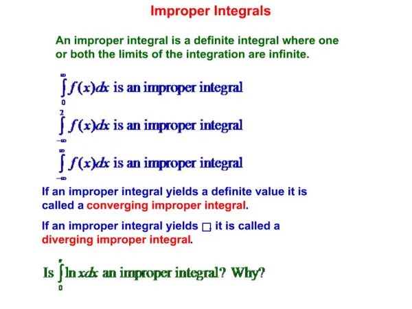
Improper Integral
Improper integral. In calculus, an improper integral is the limit of a definite integral as an endpoint of the interval of integration approaches either a specified real number or 8 or -8 or, in some cases, as both endpoints approach limits.Specifically, an improper integral is a limit of the form

Improper Integral
E N D
Presentation Transcript
1. Improper Integral Integral ambiguity,
Darbaux integral,
Lebesgue integral.
2. Improper integral In calculus, an improper integral is the limit of a definite integral as an endpoint of the interval of integration approaches either a specified real number or 8 or -8 or, in some cases, as both endpoints approach limits.
Specifically, an improper integral is a limit of the form
or of the form
in which one takes a limit in one or the other (or sometimes both) endpoints (Apostol 1967, �10.23). Improper integrals may also occur at an interior point of the domain of integration, or at multiple such points.
It is often necessary to use improper integrals in order to compute a value for integrals which may not exist in the conventional sense (as a Riemann integral, for instance) because of a singularity in the function, or an infinite endpoint of the domain of integration.
3.
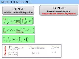
An improper integral of the first kind. The integral may need to be defined on an unbounded domain.
An improper Riemann integral of the second kind. The integral may fail to exist because of a vertical asymptote in the function.
4. Examples The following integral does not exist as a Riemann integral
because the domain of integration is unbounded. (The Riemann integral is only well-defined over a bounded domain.) However, it may be assigned a value as an improper integral by interpreting it instead as a limit
The following integral also fails to exist as a Riemann integral:
Here the function is unbounded, and the Riemann integral is not well-defined for unbounded functions. However, if the integral is instead understood as the limit:
then the limit converges.
5. Convergence of the integral An improper integral converges if the limit defining it exists. Thus for example one says that the improper integral
exists and is equal to L if the integrals under the limit exist for all sufficiently large t, and the value of the limit is equal to L.
It is also possible for an improper integral to diverge to infinity. In that case, one may assign the value of 8 (or -8) to the integral. For instance
However, other improper integrals may simply diverge in no particular direction, such as
which does not exist, even as an extended real number.
6. A limitation of the technique of improper integration is that the limit must be taken with respect to one endpoint at a time. Thus, for instance, an improper integral of the form
is defined by taking two separate limits; to wit
provided the double limit is finite. By the properties of the integral, this can also be written as a pair of distinct improper integrals of the first kind:
where c is any convenient point at which to start the integration.
7. It is sometimes possible to define improper integrals where both endpoints are infinite, such as the Gaussian integral
But one cannot even define other integrals of this kind unambiguously, such as
, since the double limit diverges:
In this case, one can however define an improper integral in the sense of Cauchy principal value:
The questions one must address in determining an improper integral are:
Does the limit exist?
Can the limit be computed?
The first question is an issue of mathematical analysis. The second one can be addressed by calculus techniques, but also in some cases by contour integration, Fourier transforms and other more advanced methods.
8. Types of integrals There is more than one theory of integration. From the point of view of calculus, the Riemann integral theory is usually assumed as the default theory. In using improper integrals, it can matter which integration theory is in play.
For the Darboux integral, improper integration is necessary both for unbounded intervals (since one cannot divide the interval into finitely many subintervals of finite length) and for unbounded functions with finite integral (since, supposing it is unbounded above, then the upper integral will be infinite, but the lower integral will be finite).
For the Riemann integral, improper integration is also necessary for unbounded intervals and for unbounded functions, as with the Darboux integral.
9. The Lebesgue integral deals differently with unbounded domains and unbounded functions, so that often an integral which only exists as an improper Riemann integral will exist as a (proper) Lebesgue integral, such as
On the other hand, there are also integrals that have an improper Riemann integral but do not have a (proper) Lebesgue integral, such as
The Lebesgue theory does not see this as a deficiency: from the point of view of measure theory,
and cannot be defined satisfactorily. In some situations, however, it may be convenient to employ improper Lebesgue integrals as is the case, for instance, when defining the Cauchy principal value.
For the Henstock�Kurzweil integral, improper integration is not necessary, and this is seen as a strength of the theory: it encompasses all Lebesgue integrable and improper Riemann integrable functions.
10. Improper Riemann integrals and Lebesgue integrals
In some cases, the integral
can be defined as an integral (a Lebesgue integral, for instance) without reference to the limit
but cannot otherwise be conveniently computed.
11. This often happens when the function f being integrated from a to c has a vertical asymptote at c, or if c�=�8 (see Figures 1 and 2). In such cases, the improper Riemann integral allows one to calculate the Lebesgue integral of the function. Specifically, the following theorem holds (Apostol 1974, Theorem 10.33):
If a function f is Riemann integrable on [a,b] for every b�=�a, and the partial integrals
are bounded as b�?�8, then the improper Riemann integrals
both exist. Furthermore, f is Lebesgue integrable on [a, 8), and its Lebesgue integral is equal to its improper Riemann integral.
12. For example, the integral
can be interpreted alternatively as the improper integral
or it may be interpreted instead as a Lebesgue integral over the set (0, 8). Since both of these kinds of integral agree, one is free to choose the first method to calculate the value of the integral, even if one ultimately wishes to regard it as a Lebesgue integral. Thus improper integrals are clearly useful tools for obtaining the actual values of integrals.
13. In other cases, however, the integral from a to c is not even defined, because the integrals of the positive and negative parts of f(x)�dx from a to c are both infinite, but nonetheless the limit may exist. Such cases are "properly improper" integrals, i.e. their values cannot be defined except as such limits. For example,
cannot be interpreted as a Lebesgue integral, since
This is therefore a "properly" improper integral, whose value is given by
.
14. Singularities One can speak of the singularities of an improper integral, meaning those points of the extended real number line at which limits are used.
Such an integral is often written symbolically just like a standard definite integral, perhaps with infinity as a limit of integration. But that conceals the limiting process. By using the more advanced Lebesgue integral, rather than the Riemann integral, one can in some cases bypass this requirement, but if one simply wants to evaluate the limit to a definite answer, that technical fix may not necessarily help. It is more or less essential in the theoretical treatment for the Fourier transform, with pervasive use of integrals over the whole real line.
15. Cauchy principal value Consider the difference in values of two limits:
The former is the Cauchy principal value of the otherwise ill-defined expression
Similarly,
16. we have
But
The former is the principal value of the otherwise ill-defined expression
All of the above limits are cases of the indeterminate form 8 - 8.
These pathologies do not affect "Lebesgue-integrable" functions, that is, functions the integrals of whose absolute values are finite.
17. Summability An indefinite integral may diverge in the sense that the limit defining it may not exist. In this case, there are more sophisticated definitions of the limit which can produce a convergent value for the improper integral. These are called summability methods.
One summability method, popular in Fourier analysis, is that of Ces�ro summation. The integral
is Ces�ro summable (C,�a) if
exists and is finite (Titchmarsh 1948, �1.15). The value of this limit, should it exist, is the (C,�a) sum of the integral.
18. An integral is (C,�0) summable precisely when it exists as an improper integral. However, there are integrals which are (C,�a) summable for a�>�0 which fail to converge as improper integrals (in the sense of Riemann or Lebesgue).
One example is the integral
which fails to exist as an improper integral, but is (C,a) summable for every a�>�0, with value 1. This is an integral version of Grandi's series.
19. Darboux integral In real analysis, a branch of mathematics, the Darboux integral or Darboux sum is one possible definition of the integral of a function. Darboux integrals are equivalent to Riemann integrals, meaning that a function is Darboux-integrable if and only if it is Riemann-integrable, and the values of the two integrals, if they exist, are equal. Darboux integrals have the advantage of being simpler to define than Riemann integrals. Darboux integrals are named after their discoverer, Gaston Darboux.
20. Definition A partition of an interval [a,b] is a finite sequence of values xi such that
Each interval [xi-1,xi] is called a subinterval of the partition. Let �:[a,b]?R be a bounded function, and let
be a partition of [a,b]. Let
Lower (green) and upper (green plus lavender) Darboux sums for four subintervals
21. The upper Darboux sum of � with respect to P is
The lower Darboux sum of � with respect to P is
The upper Darboux integral of � is
The lower Darboux integral of � is
If U��=�L�, then we say that � is Darboux-integrable and set
the common value of the upper and lower Darboux integrals.
22. Facts about the Darboux integral
When passing to a refinement, the lower sum increases and the upper sum decreases.
A refinement of the partition
is a partition
such that for every i with
there is an integer r(i) such that
In other words, to make a refinement, cut the subintervals into smaller pieces and do not remove any existing cuts. If
is a refinement of
then
and
If P1, P2 are two partitions of the same interval (one need not be a refinement of the other), then
23. It follows that
Riemann sums always lie between the corresponding lower and upper Darboux sums. Formally, if
and
together make a tagged partition
(as in the definition of the Riemann integral), and if the Riemann sum of � corresponding to P and T is R, then
From the previous fact, Riemann integrals are at least as strong as Darboux integrals: If the Darboux integral exists, then the upper and lower Darboux sums corresponding to a sufficiently fine partition will be close to the value of the integral, so any Riemann sum over the same partition will also be close to the value of the integral. It is not hard to see that there is a tagged partition that comes arbitrarily close to the value of the upper Darboux integral or lower Darboux integral, and consequently, if the Riemann integral exists, then the Darboux integral must exist as well.
24. Lebesgue integration In mathematics, Lebesgue integration refers to both the general theory of integration of a function with respect to a general measure, and to the specific case of integration of a function defined on a sub-domain of the real line or a higher dimensional Euclidean space with respect to the Lebesgue measure. This article focuses on the more general concept.
Lebesgue integration plays an important role in real analysis, the axiomatic theory of probability, and many other fields in the mathematical sciences.
The integral of a non-negative function can be regarded in the simplest case as the area between the graph of that function and the x-axis. The Lebesgue integral is a construction that extends the integral to a larger class of functions defined over spaces more general than the real line.
For non-negative functions with a smooth enough graph (such as continuous functions on closed bounded intervals), the area under the curve is defined as the integral and computed using techniques of approximation of the region by polygons (see Simpson's rule). For more irregular functions (such as the limiting processes of mathematical analysis and probability theory), better approximation techniques are required in order to define a suitable integral.
25. Introduction The integral of a function f between limits a and b can be interpreted as the area under the graph of f. This is easy to understand for familiar functions such as polynomials, but what does it mean for more exotic functions? In general, what is the class of functions for which "area under the curve" makes sense? The answer to this question has great theoretical and practical importance.
As part of a general movement toward rigour in mathematics in the nineteenth century, attempts were made to put the integral calculus on a firm foundation. The Riemann integral, proposed by Bernhard Riemann (1826�1866), is a broadly successful attempt to provide such a foundation. Riemann's definition starts with the construction of a sequence of easily-calculated areas which converge to the integral of a given function. This definition is successful in the sense that it gives the expected answer for many already-solved problems, and gives useful results for many other problems. However, Riemann integration does not interact well with taking limits of sequences of functions, making such limiting processes difficult to analyze. This is of prime importance, for instance, in the study of Fourier series, Fourier transforms and other topics. The Lebesgue integral is better able to describe how and when it is possible to take limits under the integral sign. The Lebesgue definition considers a different class of easily-calculated areas than the Riemann definition, which is the main reason the Lebesgue integral is better behaved. The Lebesgue definition also makes it possible to calculate integrals for a broader class of functions. For example, the Dirichlet function, which is 0 where its argument is irrational and 1 otherwise, has a Lebesgue integral, but it does not have a Riemann integral.
26. Construction of the Lebesgue integral Measure theory
Measure theory was initially created to provide a useful abstraction of the notion of length of subsets of the real line and, more generally, area and volume of subsets of Euclidean spaces. In particular, it provided a systematic answer to the question of which subsets of R have a length. As was shown by later developments in set theory (see non-measurable set), it is actually impossible to assign a length to all subsets of R in a way which preserves some natural additivity and translation invariance properties. This suggests that picking out a suitable class of measurable subsets is an essential prerequisite.
The Riemann integral uses the notion of length explicitly. Indeed, the element of calculation for the Riemann integral is the rectangle [a,�b]�נ[c,�d], whose area is calculated to be (b�-�a)(d�-�c). The quantity b�-�a is the length of the base of the rectangle and d�-�c is the height of the rectangle. Riemann could only use planar rectangles to approximate the area under the curve because there was no adequate theory for measuring more general sets.
In the development of the theory in most modern textbooks (after 1950), the approach to measure and integration is axiomatic. This means that a measure is any function � defined on a certain class X? of subsets of a set E, which satisfies a certain list of properties. These properties can be shown to hold in many different cases.
27. Integration
We start with a measure space (E,�X,��) where E is a set, X is a s-algebra of subsets of E and � is a (non-negative) measure on X of subsets of E.
For example, E can be Euclidean n-space Rn or some Lebesgue measurable subset of it, X will be the s-algebra of all Lebesgue measurable subsets of E, and � will be the Lebesgue measure. In the mathematical theory of probability, we confine our study to a probability measure��, which satisfies �(E) = 1.
In Lebesgue's theory, integrals are defined for a class of functions called measurable functions. A function � is measurable if the pre-image of every closed interval is in X:
It can be shown that this is equivalent to requiring that the pre-image of any Borel subset of R be in X. We will make this assumption henceforth. The set of measurable functions is closed under algebraic operations, but more importantly the class is closed under various kinds of pointwise sequential limits:
are measurable if the original sequence (�k)k, where k�? N, consists of measurable functions.
28. We build up an integral
for measurable real-valued functions � defined on E in stages:
Indicator functions: To assign a value to the integral of the indicator function of a measurable set S consistent with the given measure �, the only reasonable choice is to set:
Notice that the result may be equal to +8, unless � is a finite measure.
Simple functions: A finite linear combination of indicator functions
where the coefficients ak are real numbers and the sets Sk are measurable, is called a measurable simple function.
29. We extend the integral by linearity to non-negative measurable simple functions. When the coefficients ak are non-negative, we set
The convention 0�נ8�= 0 must be used, and the result may be infinite. Even if a simple function can be written in many ways as a linear combination of indicator functions, the integral will always be the same.
Some care is needed when defining the integral of a real-valued simple function, in order to avoid the undefined expression 8�-�8: one assumes that the representation
is such that �(Sk)�< 8 whenever ak�?�0. Then the above formula for the integral of � makes sense, and the result does not depend upon the particular representation of � satisfying the assumptions.
30. If B is a measurable subset of E and s a measurable simple function one defines
Non-negative functions: Let � be a non-negative measurable function on E which we allow to attain the value +8, in other words, � takes non-negative values in the extended real number line. We define
We need to show this integral coincides with the preceding one, defined on the set of simple functions. When E? is a segment [a,�b], there is also the question of whether this corresponds in any way to a Riemann notion of integration. It is possible to prove that the answer to both questions is yes.
We have defined the integral of � for any non-negative extended real-valued measurable function on�E. For some functions, this integral? ?E���d�? will be infinite.
31. Signed functions: To handle signed functions, we need a few more definitions. If � is a measurable function of the set E to the reals (including � 8), then we can write
Where
Note that both �+ and �- are non-negative measurable functions. Also note that
If
then � is called Lebesgue integrable. In this case, both integrals satisfy
and it makes sense to define
It turns out that this definition gives the desirable properties of the integral.
Complex valued functions can be similarly integrated, by considering the real part and the imaginary part separately.
32. Intuitive interpretation To get some intuition about the different approaches to integration, let us imagine that it is desired to find a mountain's volume (above sea level).
The Riemann-Darboux approach: Divide the base of the mountain into a grid of 1 meter squares. Measure the altitude of the mountain at the center of each square. The volume on a single grid square is approximately 1x1x(altitude), so the total volume is the sum of the altitudes.
The Lebesgue approach: Draw a contour map of the mountain, where each contour is 1 meter of altitude apart. The volume of earth contained in a single contour is approximately that contour's area times its height. So the total volume is the sum of these volumes.
Folland summarizes the difference between the Riemann and Lebesgue approaches thus: "to compute the Riemann integral of f, one partitions the domain [a,�b] into subintervals", while in the Lebesgue integral, "one is in effect partitioning the range of f".
33. Example Consider the indicator function of the rational numbers, 1Q. This function is nowhere continuous.
1Q is not Riemann-integrable on [0,1]: No matter how the set [0,1] is partitioned into subintervals, each partition will contain at least one rational and at least one irrational number, since rationals and irrationals are both dense in the reals. Thus the upper Darboux sums will all be one, and the lower Darboux sums will all be zero.
1Q is Lebesgue-integrable on [0,1] using the Lebesgue measure: Indeed it is the indicator function of the rationals so by definition
since Q is countable.
34. Limitations of the Riemann integral Here we discuss the limitations of the Riemann integral and the greater scope offered by the Lebesgue integral. We presume a working understanding of the Riemann integral.
With the advent of Fourier series, many analytical problems involving integrals came up whose satisfactory solution required interchanging limit processes and integral signs. However, the conditions under which the integrals
and
are equal proved quite elusive in the Riemann framework. There are some other technical difficulties with the Riemann integral. These are linked with the limit taking difficulty discussed above.
35. Failure of monotone convergence. As shown above, the indicator function 1Q on the rationals is not Riemann integrable. In particular, the Monotone convergence theorem fails. To see why, let {ak} be an enumeration of all the rational numbers in [0,1] (they are countable so this can be done.) Then let
The function gk is zero everywhere except on a finite set of points, hence its Riemann integral is zero. The sequence gk is also clearly non-negative and monotonically increasing to 1Q, which is not Riemann integrable.
Unsuitability for unbounded intervals. The Riemann integral can only integrate functions on a bounded interval. It can however be extended to unbounded intervals by taking limits, so long as this doesn't yield an answer such as .
What about integrating on structures other than Euclidean space? The Riemann integral is inextricably linked to the order structure of the line. How do we free ourselves of this limitation?