Polynomial Regression for Biological Data Analysis
Learn how to model nonlinear data in biology using polynomial regression and model selection criteria.

Polynomial Regression for Biological Data Analysis
E N D
Presentation Transcript
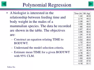
Polynomial Regression • A biologist is interested in the relationship between feeding time and body weight in the males of a mammalian species. The data he recorded are shown in the table. The objectives are: • Construct an equation relating TIME to BODYWT. • Understand the model selection criteria. • Estimate mean TIME for a given BODYWT with 95% CLM.
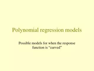
The Relationship Is Nonlinear Y = a + b X ? Y = a eX ? Y = a Xb ?
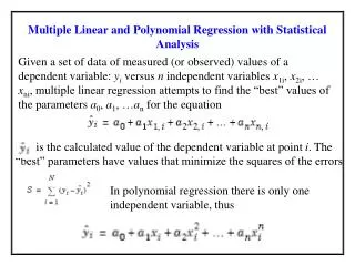
Polynomial Regression • Polynomial regression is a special type of multiple regression whose independent variables are powers of a single variable X. It is used to approximate a curve with unknown functional form.Yi = + 1 X + 2 X2 + … + k Xk + i • Model selection is done by successively testing highest order terms and discarding insignificant highest-order terms. Tests should use a liberal level of significance, such as = 0.25. The starting order should usually be k < N/10, where N is the number of observations.
Polynomial Regression • The main reason for successively testing/discarding highest degree terms and discarding insignificant terms is because the higher order terms are more prone to random error in X, i.e, the random error is multiplied several times in higher order terms. • Suppose the true value for X is 2 but, because of measurement error, we obtain a value of 3. X2 is then 9. If we had measured the X value accurately, the X2 value would have been 4. So the value of 9 obtained is 4 + 5 units of error. X3 = 27 = 8 + 19 units of error. • Thus, if an order-4 regression is not significantly better than an order-3 regression, then the X4 term is dropped. • Contrast with the model selection in multiple regression with X1, X2, etc.
Polynomial Regression (order 6) If you keep increasing the number of polynomial terms in the equation, eventually you will have perfect fit. Is that what you want?
Do the Test in SAS data polydat; input FeedTime BodyWt @@; BodyWt2=BodyWt*BodyWt; BodyWt3=BodyWt2*BodyWt; BodyWt4=BodyWt3*BodyWt; cards; 1.22 40.9 2.14 44.3 2.39 44.7 3.50 48.6 1.66 43.0 2.97 45.4 3.95 50.0 1.34 41.8 2.51 45.0 3.53 49.0 1.72 43.4 3.17 46.2 4.11 50.8 1.51 42.4 2.78 45.1 3.85 49.7 1.93 43.9 3.32 47.0 4.18 51.1 ; proc glm; model FeedTime=BodyWt BodyWt2 BodyWt3/SS1; run; proc glm; model FeedTime=BodyWt BodyWt2/ss1 p clm; run;
SAS Output Dependent Variable: FEEDTIME Source DF Sum of Squares F Value Pr > F Model 3 17.16627141 197.13 0.0001 Error 15 0.43540228 Corrected Total 18 17.60167368 R-Square C.V. FEEDTIME Mean 0.975264 6.251601 2.72526316 Source DF Type I SS F Value Pr > F BODYWT 1 16.93053484 583.27 0.0001 BODYWT2 1 0.17828754 6.14 0.0256 BODYWT3 1 0.05744902 1.98 0.1799
SAS Output: order of 3 T for H0: Pr>|T| Std Error of Parameter Estimate Parameter=0 Estimate INTERCEPT 197.5414064 1.19 0.2533 166.2638449 BODYWT -13.9642883 -1.28 0.2200 10.9105501 BODYWT2 0.3234063 1.36 0.1945 0.2381090 BODYWT3 -0.0024311 -1.41 0.1799 0.0017280 T-Test here is equivalent to F-test based on Type II SS (Type II, Type III and Type IV are all the same in regression). Note: T-tests give misleading results for polynomial models. For our data, all t-tests are nonsignificant, which is clearly misleading. Why? (Hint: what models are the t-tests comparing?)
SAS output: Order of 2 Dependent Variable: FEEDTIME Source DF Sum of Squares F Value Pr > F Model 2 17.10882239 277.71 0.0001 Error 16 0.49285130 Corrected Total 18 17.60167368 Source DF Type I SS F Value Pr > F BODYWT 1 16.93053484 549.64 0.0001 BODYWT2 1 0.17828754 5.79 0.0286 T for H0: Pr>|T| Std Error of Parameter Estimate Parameter=0 Estimate INTERCEPT -35.94660928 -3.52 0.0029 10.22189563 BODYWT 1.37306931 3.10 0.0069 0.44306000 BODYWT2 -0.01150885 -2.41 0.0286 0.00478376 Feeding Time = -35.947 + 1.373 BodyWt - 0.012 BodyWt2 Hand-compute the adjusted R2 for the two polynomial regressions (i.e., order 3 and order 2) and decide whether X3 should be kept or discarded.
Prediction Observation Observed Predicted Residual 1 1.22000000 0.95980313 0.26019687 2 2.14000000 2.29435461 -0.15435461 3 2.39000000 2.43386721 -0.04386721 4 3.50000000 3.60111164 -0.10111164 5 1.66000000 1.81550409 -0.15550409 6 2.97000000 2.66915245 0.30084755 7 3.95000000 3.93472678 0.01527322 ...... 95% Confidence Limits for Observation Mean Predicted Value 1 0.70344686 1.21615939 2 2.18244285 2.40626636 3 2.31762886 2.55010556 4 3.47982526 3.72239801 ......