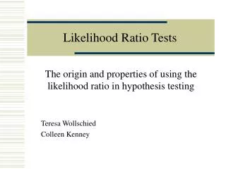
Likelihood Ratio Tests: Origin and Properties in Hypothesis Testing
310 likes | 384 Vues
Explore the history and application of likelihood ratio tests in hypothesis testing, with insights into Neyman and Pearson's contributions and the statistical concepts involved.

Likelihood Ratio Tests: Origin and Properties in Hypothesis Testing
E N D
Presentation Transcript
Likelihood Ratio Tests The origin and properties of using the likelihood ratio in hypothesis testing Teresa Wollschied Colleen Kenney
Outline • Background/History • Likelihood Function • Hypothesis Testing • Introduction to Likelihood Ratio Tests • Examples • References
Jerzy Neyman (1894 – 1981) • Jerzy Neyman (1894 – 1981) • April 16, 1894: Born in Benderry, Russia/Moldavia (Russian version:Yuri Czeslawovich) • 1906: Father died. Neyman and his mother moved to Kharkov. • 1912:Neyman began study in both physics and mathematics at University of Kharkov where professor Aleksandr Bernstein introduced him to probability • 1919: Traveled south to Crimea and met Olga Solodovnikova. In 1920 ten days after their wedding, he was imprisoned for six weeks in Kharkov. • 1921: Moved to Poland and worked as an asst. statistical analyst at the Agricultural Institute in Bromberg then State Meteorological Institute in Warsaw.
Neyman biography • 1923-1924:Became an assistant at Warsaw University and taught at the College of Agriculture. Earned a doctorate for a thesis that applied probability to agricultural experimentation. • 1925: Received the Rockefeller fellowship to study at University College London with Karl Pearson (met Egon Pearson) • 1926-1927:Went to Paris. Visited by Egon Pearson in 1927, began collaborative work on testing hypotheses. • 1934-1938: Took position at University College London • 1938: Offered a position at UC Berkeley. Set up Statistical Laboratory within Department of Mathematics. Statistics became a separate department in 1955. • Died on August 5, 1981
Egon Pearson (1895 – 1980) • August 11, 1895: Born in Hampstead, England. Middle child of Karl Pearson • 1907-1909: Attended Dragon School Oxford • 1909-1914: Attended Winchester College • 1914: Started at Cambridge, interrupted by influenza. • 1915: Joined war effort at Admiralty and Ministry of Shipping • 1920: Awarded B.A. by taking Military Special Examination; Began research in solar physics, attending lectures by Eddington • 1921: Became lecturer at University College London with his father • 1924: Became assistant editor of Biometrika
Pearson biography • 1925: Met Neyman and corresponded with him through letters while Neyman was in Paris. Also corresponded with Gosset at the same time. • 1933: After father retires, becomes the Head of Department of Apllied Statistics • 1935: Won Weldon Prize for work done with Neyman and began work on revising Tables for Statisticians and Biometricians (1954,1972) • 1939: Did war work, eventually receiving a C.B.E. • 1961: Retired from University College London • 1966: Retired as Managing Editor of Biometrika • Died June 12, 1890
Likelihood and Hypothesis Testing • “On The Use and Interpretation of Certain Test Criteria for Purposes of Statistical Inference, Part I,” 1928, Biometrika: Likelihood Ratio Tests explained in detail by Neyman and Pearson • “Probability is a ratio of frequencies and this relative measure cannot be termed the ratio of probabilities of the hypotheses, unless we speak of probability a posteriori and postulate some a priori frequency distribution of sampled populations. Fisher has therefore introduced the term likelihood, and calls this comparative measure the ratio of the two hypotheses.
Likelihood and Hypothesis Testing • “On the Problem of the most Efficient Tests of Statistical Hypotheses,” 1933, Philosophical Transactions of the Royal Society of London: The concept of developing an ‘efficient’ test is expanded upon. • “Without hoping to know whether each hypothesis is true or false, we may search for rules to govern our behavior with regard to them, in following which we insure that, in the long run of experience, we shall not be too often wrong”
Hypothesis Testing • Define T=r(x) • R={x: T>c} for some constant c.
Power Function • The probability a test will reject H0 is given by: • Size test: • Level test:
Types of Error • Type I Error: Rejecting H0 when H0 is true • Type II Error: Accepting H0 when H0 is false
Likelihood Ratio Test (LRT) • LRT statistic for testing H0: 0 vs. Ha: a is: • A LRT is any test that has a rejection region of the form {x: (x) c}, where c is any number such that 0 c 1.
Uniformly Most Powerful (UMP) Test • Let be a test procedure for testing H0: 0 vs. Ha: a, with level of significance 0.Then , with power function (), is a UMP level 0 test if: • () 0 • For every test procedure ′ with (′) 0, we have′() () for every a.
Neyman-Pearson Lemma Consider testing H0: = 0 vs. Ha: = 1, where the pdf or pmf corresponding to i is f(x|i), i=0,1, using a test with rejection region R that satisfies xR if f(x|1) > k f(x|0) (1) and xRc if f(x|1) < k f(x|0), for some k 0, and (2)
Neyman-Pearson Lemma (cont’d) • Then • Any test that satisfies (1) and (2) is a UMP level test. • If there exists a test satisfying (1) and (2) with k>0, then every UMP level test satisfies (2) and every UMP level test satisfies (1) except perhaps on a set A satisfying
Example: Normal LRT (cont’d) • We will reject H0 if (x) c. We have: • Therefore, the LRTs are those tests that reject H0 if the sample mean differs from the value 0 by more than
Sufficient Statistics and LRTs Theorem: If T(X) is a sufficient statistic for , and *(t) and (t) are the LRT statistics based on T and X, respectively, then *(T(x))=(x) for every x in the sample space.
Restrictions • When a UMP test does not exist, other methods must be used. • Consider subset of tests and search for a UMP test.
References Cassella, G. and Berger, R.L. (2002). Statistical Inference. Duxbury:Pacific Grove, CA. Neyman, J. and Pearson, E., “On The Use and Interpretation of Certain Test Criteria for Purposes of Statistical Inference, Part I,” Biometrika, Vol. 20A, No.1/2 (July 1928), pp.175-240. Neyman, J. and Pearson, E., “On the Problem of the most Efficient Tests of Statistical Hypotheses,” Philosophical Transactions of the Royal Society of London, Vol. 231 (1933), pp. 289-337. http://www-history.mcs.st-andrews.ac.uk/Mathematicians/Pearson_Egon.html http://www-history.mcs.st-andrews.ac.uk/Mathematicians/Neyman.html