Download
1 / 89
890 likes | 1.15k Vues
Introduction to Gene-Finding: Linkage and Association. Danielle Dick, Sarah Medland, (Ben Neale). Aim of QTL mapping…. LOCALIZE and then IDENTIFY a locus that regulates a trait (QTL)

E N D
Introduction to Gene-Finding: Linkage and Association Danielle Dick, Sarah Medland, (Ben Neale)
Aim of QTL mapping… LOCALIZE and then IDENTIFY a locus that regulates a trait (QTL) • Locus: Nucleotide or sequence of nucleotides with variation in the population, with different variants associated with different trait levels.
Location and Identification • Linkage • localize region of the genome where a QTL that regulates the trait is likely to be harboured • Family-specific phenomenon: Affected individuals in a family share the same ancestral predisposing DNA segment at a given QTL
Location and Identification • Association • identify a QTL that regulates the trait • Population-specific phenomenon: Affected individuals in a population share the same ancestral predisposing DNA segment at a given QTL
Linkage Overview
Progress of the Human Genome Project Human Chromosome 4
Genetic markers (DNA polymorphisms) ATGCTTGCCACGCE ATGCTTCTTGCCATGCE Microsatellite Markers can be di(2), tri(3), or tetra (4) nucleotide repeats ATGCTTGCCACGCE ATGCTTGCCATGCE Single Nucleotide Polymorphism
DNA polymorphisms • Can occur in gene, but be silent • Can change gene product (protein) • Alter amino acid sequence (a lot or a little) • Can regulate gene product • Upregulate or downregulate protein production • Turn off or on gene • Can occur in noncoding region • This happens most often!
How do we map genes? • Deviation from Mendel’s Independent Assortment Law • Aa & Bb = ¼ AB, ¼ Ab, ¼ aB, ¼ ab • We’re looking for variation from this
Recombination • Another way of introducing genetic diversity • Allows us to map genes! • Crossovers more likely to occur between genes that are further away; likelihood of a recombination event is proportional to the distance • Interference – tend not to see 2 crossovers in a small area • Alleles that are very close together are more likely to stay together, don’t assort independently
Linkage Mapping (is a marker “linked” to the disease gene) • Collect families with affected individuals • Genome Scan - Test markers evenly spaced across the entire genome (~every 10cM, ~400 markers) • Lod score (“log of the odds”) – what are the odds of observing the family marker data if the marker is linked to the disease (less recombination than expected) compared to if the marker is not linked to the disease
Linkage = Co-segregation A3A4 A1A2 A1A3 A2A4 A2A3 Marker allele A1 cosegregates with dominant disease A1A2 A1A4 A3A4 A3A2
Lod scores • >3.0 evidence for linkage • <-2.0 can rule out linkage • In between – inconclusive, collect more families
Linkage = Co-segregation • Parametric Linkage used very successfully to map disease genes for Mendelian disorders • Problematic for complex disorders: requires disease model, penetrance, assumes gene of major effect, phenotypic precision A3A4 A1A2 A1A3 A2A4 A2A3 A1A2 A1A4 A3A4 A3A2
Nonparametric Linkage • Based on allele-sharing • More appropriate for phenotypes with multiple genes of small effect, environment, no disease model assumed • Basic unit of data: affected relative (often sibling) pairs
x 1/4 1/4 1/4 1/4
IDENTITY BY DESCENT Sib 1 2 1 1 0 1 2 0 1 Sib 2 1 0 2 1 0 1 1 2 4/16 = 1/4 sibs share BOTH parental alleles IBD = 2 8/16 = 1/2 sibs share ONE parental allele IBD = 1 4/16 = 1/4 sibs share NO parental alleles IBD = 0
Genotypic similarity between relatives IBSAlleles shared Identical By State “look the same”, may have the same DNA sequence but they are not necessarily derived from a known common ancestor - focus for association M3 M1 M2 M3 Q3 Q1 Q2 Q4 IBDAlleles shared Identical By Descent are a copy of the same ancestor allele - focus for linkage M1 M2 M3 M3 Q1 Q2 Q3 Q4 IBD IBS M1 M3 M1 M3 2 1 Q1 Q4 Q1 Q3
Genotypic similarity – basic principals • Loci that are close together are more likely to be inherited together than loci that are further apart • Loci are likely to be inherited in context – ie with their surrounding loci • Because of this, knowing that a loci is transmitted from a common ancestor is more informative than simply observing that it is the same allele • Critical to have parental data when possible
For disease traits (affected/unaffected) Affected sib pairs selected 1000 750 500 250 IBD = 2 Expected 1 2 3 127 310 IBD = 1 Markers IBD = 0
1.00 0.75 Correlation between sibs 0.50 0.25 0.00 IBD = 0 IBD = 1 IBD = 2 For continuous measures Unselected sib pairs
IDENTITY BY DESCENT Sib 1 2 1 1 0 1 2 0 1 Sib 2 1 0 2 1 0 1 1 2 4/16 = 1/4 sibs share BOTH parental alleles IBD = 2 8/16 = 1/2 sibs share ONE parental allele IBD = 1 4/16 = 1/4 sibs share NO parental alleles IBD = 0
In biometrical modeling A is correlated at 1 for MZ twins and .5 for DZ twins • .5 is the average genome-wide sharing of genes between full siblings (DZ twin relationship)
In linkage analysis we will be estimating an additional variance component Q • For each locus under analysis the coefficient of sharing for this parameter will vary for each pair of siblings • The coefficient will be the probability that the pair of siblings have both inherited the same alleles from a common ancestor
MZ=1.0 DZ=0.5 MZ & DZ = 1.0 1 1 1 1 1 1 1 1 Q A C E E C A Q e c a q q a c e PTwin1 PTwin2
Linkage How do we do this? 1.Genotyping data.
Microsatellite data • Ideally positioned at equal genetic distances across chromosome • Mostly di/tri nucleotide repeats http://research.marshfieldclinic.org/genetics/GeneticResearch/screeningsets.asp
Microsatellite data • Raw data consists of allele lengths/calls (bp) • Different primers give different lengths • So to compare data you MUST know which primers were used http://research.marshfieldclinic.org/genetics/GeneticResearch/screeningsets.asp
Binning • Raw allele lengths are converted to allele numbers or lengths • Example:D1S1646 tri-nucleotide repeat size range130-150 • Logically: Work with binned lengths • Commonly: Assign allele 1 to 130 allele, 2 to 133 allele … • Commercially: Allele numbers often assigned based on reference populations CEPH. So if the first CEPH allele was 136 that would be assigned 1 and 130 & 133 would assigned the next free allele number • Conclusions: whenever possible start from the RAW allele size and work with allele length
Error checking • After binning check for errors • Family relationships (GRR, Rel-pair) • Mendelian Errors (Sib-pair) • Double Recombinants (MENDEL, ASPEX, ALEGRO) • An iterative process
‘Clean’ data • ped file • Family, individual, father, mother, sex, dummy, genotypes
Estimating genotypic sharing… • The ped file is used with ‘map’ files to obtain estimates of genotypic sharing between relatives at each of the locations under analysis
Estimating genotypic sharing… Merlin will give you probabilities of sharing 0, 1, 2 alleles for every pair of individuals.
Estimating genotypic sharing… • Output
Estimating genotypic sharing… • Output Why isn’t P0, P1, P2 exact for everyone?
Estimating genotypic sharing… • Output Why isn’t P0, P1, P2 exact for everyone? -missing parental genotypes -low informativeness at marker 1/2 2/2 2/2 1/2
MZ=1.0 DZ=0.5 MZ & DZ = 1.0 1 1 1 1 1 1 1 1 Q A C E E C A Q e c a q q a c e PTwin1 PTwin2
Genotypic similarity between relatives IBDAlleles shared Identical By Descent are a copy of the same ancestor allele Pairs of siblings may share 0, 1 or 2 alleles IBD The probability of a pair of relatives being IBD is known as pi-hat M3 M1 M2 M3 Q3 Q1 Q2 Q4 M1 M2 M3 M3 Q1 Q2 Q3 Q4 IBS IBD M1 M3 M1 M3 2 1 Q1 Q4 Q1 Q3
Estimating genotypic sharing… • Output
Distribution of pi-hat • Adult Dutch DZ pairs: distribution of pi-hat at 65 cM on chromosome 19 • < 0.25: IBD=0 group • > 0.75: IBD=2 group • others: IBD=1 group • pi65cat= (0,1,2)
Linkage Analyses • Advantage • Systematically scan the genome • Disadvantages • Not very powerful • Need hundreds – thousands of family member • Broad peaks
Lod scores 1cM = 1MB 1MB=1000kb 1kb=1000bp 1cM = 1,000,000 bp
Strategy 1. Ascertain families with multiple affecteds 2. Linkage analyses to identify chromosomal regions allele-sharing among affecteds within a family 3. Association analyses to identify specific genes Gene A Gene B Gene C
Linkage vs. Association • Linkage analyses look for relationship between a marker and disease within a family (could be different marker in each family) • Association analyses look for relationship between a marker and disease between families (must be same marker in all families)