Download
1 / 29
290 likes | 319 Vues
Learn about the fundamental concepts of graphs, paths, cycles, and data structures for representing graphs. Understand how graphs are used to solve real-world problems efficiently. Contact Brian Mitchell for more information.

E N D
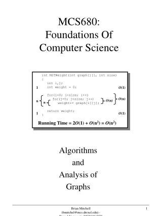
int MSTWeight(int graph[][], int size) { int i,j; int weight = 0; for(i=0; i<size; i++) for(j=0; j<size; j++) weight+= graph[i][j]; return weight; } 1 1 O(1) O(1) O(n) O(n) n n Running Time = 2O(1) + O(n2) = O(n2) MCS680:Foundations Of Computer Science Algorithms and Analysis of Graphs Brian Mitchell (bmitchel@mcs.drexel.edu) - Drexel University MCS680-FCS
Introduction • Graphs are a versatile model for organizing data • Graphs are commonly used to model many “real world” problems • Computing distances • Network routing • Reliability analysis • Finding circularities in relationships • Optimization analysis • A graph is a binary relation • Graphs can be naturally visualized • Graphs come in several forms • Directed, Undirected, Labeled • Many useful algorithms have been developed using graphs Brian Mitchell (bmitchel@mcs.drexel.edu) - Drexel University MCS680-FCS
Graph Concepts • A directed graph consists of • A set N of nodes • A binary relation A on N. • A is the set of arcs in a directed graph • An arc is a pair of nodes • Example directed graph • A = {(1,1), (1,2), (1,3), (2,4), (3,1), (3,2), (3,5), (4,3), (4,5), (5,2)} • Each pair (u,v) in A is represented by an arrow from u to v. Also noted as u v. 1 2 3 4 5 Brian Mitchell (bmitchel@mcs.drexel.edu) - Drexel University MCS680-FCS
Paths and Cycles In Graphs • A path in a directed graph is a list of nodes {v1, v2, ... , vn} such as there is an arc from node vi to node vi+1 for i = 1, 2, ... k-1 • The length of the path is k-1 which is the number of arcs along the path • Unlike trees, graphs may have cycles • A cycle is defined as a path of length 1 or more that begins and ends at the same node • The length of a cycle is the length of the path that begins and ends at the same node • The following graph has many cycles CYCLES (1,1) (1,3,1) (1,2,4,3,1) (2,4,3,2) (2,4,5,2) There are many others 1 2 3 4 5 Brian Mitchell (bmitchel@mcs.drexel.edu) - Drexel University MCS680-FCS
Undirected Graphs • Sometimes it makes sense to connect nodes in a graph by lines that have no direction • These lines are called edges • Assumed to be bi-directional • The edge {u, v} says that nodes u and v are connected in both directions • Given edge {u, v} we can say that the nodes are adjacent or neighbors • Directed edges such as u v means that node u is a predecessor of node v, and that node v is a successor of node u Router Engineers Network Computer Room Internet Production Network Brian Mitchell (bmitchel@mcs.drexel.edu) - Drexel University MCS680-FCS
Paths and Cycles in Undirected Graphs • A path in an undirected graph is defined the same way as it was in a directed graph • A path in a undirected graph is a list of nodes {v1, v2, ... , vn} such as there is an arc from node vi to node vi+1 for i = 1, 2, ... k-1 • The length of the path is k-1 which is the number of arcs along the path • A cycle in an undirected graph is a little hard to define • Because edges are bi-directional we can say that given {u, v}, that there is a cycle from u v u • This is generally not desired • A simple cycle in a directed graph is defined as a cycle that has a path of length 3 or more and that no node is repeated in the cycle with the exception of the first and last node in the cycle. Brian Mitchell (bmitchel@mcs.drexel.edu) - Drexel University MCS680-FCS
Data Structures for Representing Graphs • There are two common data structures for representing graphs • Adjacency Lists: Good sparse graphs • An array of linked lists where each position in the array represents a node, and each linked list represents the set of edges originating from the node • Efficient use of space • Slow for accessing edge information • Adjacency Matrices: Good for dense graphs • A two-dimensional array where index A[i,j] is used to indicate if an edge exists between node i, and node j • Fast access to edge information • Waste a lot of space in sparsely connected graphs • Some algorithms are optimized for either an adjacency list or an adjacency matrix representation Brian Mitchell (bmitchel@mcs.drexel.edu) - Drexel University MCS680-FCS
Adjacency List and Adjacency Matrix Representation of Graphs 1 2 3 4 5 Adjacency List Adjacency Matrix 1 1 2 3 4 5 1 1 0 1 0 0 2 1 0 0 0 1 3 1 0 0 1 0 4 0 1 0 0 0 5 0 0 1 1 0 1 2 3 2 4 3 1 5 4 3 5 5 2 Note: In order to represent an undirected graph, add nodes to the adjacency list for u v and for v u. For an adjacency matrix representation add a ‘1’ to A[i,j] and A[j,i] Brian Mitchell (bmitchel@mcs.drexel.edu) - Drexel University MCS680-FCS
Weighted Graphs • Sometimes we want to label the edges in a graph with weights • The weights are used as a measure of “capacity” of the edge • Example: Link bandwidth in a communication network • Example: The cost of transporting merchandise between two cities • Support for weighted graphs • Adjacency Lists • Each node in the adjacency list not only contains the destination node, but it also is augmented with the weight of the edge • Adjacency Matrix • Instead of using a one (‘1’) to represent an edge, use the weight of the edge instead • Use a weight of zero (‘0’) to indicate that no edge exists between two nodes in the adjacency matrix Brian Mitchell (bmitchel@mcs.drexel.edu) - Drexel University MCS680-FCS
Degree of Graphs and Graph Nodes • Directed Graphs • The number of arcs out of a node u, is called the out-degree of node u • The number of arcs into a node v, is called the in-degree of node v • Undirected Graphs • The degree of node u in an undirected graph is defined as the number of neighbors of node u • Degrees of Entire Graphs • The out-degree of a directed graph is the maximum out-degree of all nodes in the directed graph • The in-degree of a directed graph is the maximum in-degree of all nodes in the directed graph • The degree of an undirected graph is the maximum degree of all nodes in the undirected graph Brian Mitchell (bmitchel@mcs.drexel.edu) - Drexel University MCS680-FCS
Degree of Graph and Graph Nodes Using Data Structures • Directed Graphs • The length of the adjacency list is the out-degree of a node in an adjacency list. • The number of 1’s in a row in an adjacency matrix is the out-degree of the node • The number of 1’s in a column of an adjacency matrix is the in-degree of the node • There is no easy way to determine the in-degree of a node using an adjacency list • Undirected Graphs • The length of the adjacency list is the degree of the node • The number of 1’s in a row in an adjacency matrix is the degree of the node Brian Mitchell (bmitchel@mcs.drexel.edu) - Drexel University MCS680-FCS
Connected Components of an Undirected Graph • Goal • To divide an undirected graph into one or more connected components • Each connected component is a set of nodes with paths from any member in the component to any other • A connected component does not have any edges to nodes that are outside the connected component • If a graph contains a single connected component then we say that it is connected 1 2 6 7 This graph has two connected components 3 4 8 9 5 Brian Mitchell (bmitchel@mcs.drexel.edu) - Drexel University MCS680-FCS
Algorithm For Determining Connected Components • Take each node in the original graph G and make new graphs G0, G1, ... Gn-1 where each graph Gi (i = 0...n) is a graph consisting of a single node and no edges • Now consider the edges {u, v} in the original graph G. • If nodes u and v are in the same connected components then do nothing • If nodes u and v are in different connected components then merge the connected components containing u and v into a single connected component • In order to implement this algorithm we need an efficient way to: • Find the component associated with a given node (use a tree follow node to root) • Merge two distinct components into a single component (merge roots of components) Brian Mitchell (bmitchel@mcs.drexel.edu) - Drexel University MCS680-FCS
Spanning Trees • Unrooted Trees • An unrooted tree is a tree with no node designated as the root • There is no notion of children of a node or order among the children • An unrooted tree is a graph that has no simple cycles • Spanning Trees • A spanning tree for graph G consists of • The set of nodes V in G • A subset of the edges E in G that • Connect all of the nodes in V • Form an unordered, unrooted tree 1 2 1 2 Notice that many other spanning trees might exist for G 3 4 3 4 Brian Mitchell (bmitchel@mcs.drexel.edu) - Drexel University MCS680-FCS
Minimum Spanning Trees • If G is a single connected component, then there is always a spanning tree. A minimal spanning tree is a spanning tree however • The sum of the weights of the edges in the minimum spanning tree is as small as that of any spanning tree for the given graph 8 7 b c d 9 4 2 4 14 a 11 i e 6 7 8 10 h g f 1 2 Brian Mitchell (bmitchel@mcs.drexel.edu) - Drexel University MCS680-FCS
Finding a Minimum Spanning Tree • Kruskal’s Algorithm • Extension to the connected component algorithm • Take each node in the original graph G and make new graphs G0, G1, ... Gn-1 where each graph Gi (i = 0...n) is a graph consisting of a single node and no edges • Now consider the edges {u, v} in the original graph G in sorted order • If nodes u and v are in the same connected components then do nothing • If nodes u and v are in different connected components then merge the connected components containing u and v into a single connected component Brian Mitchell (bmitchel@mcs.drexel.edu) - Drexel University MCS680-FCS
Minimum Spanning Tree Example b c d a i e h g f 1: g,h 2: g,f & i,c 4: a,b & c,f 6: i,g 7: i,h & c,d 8: a,h & b,c 9: d,e 10: f,e 11: b,h 14: d,f b c d a i e h g f 1 b c d 2 a i e h g f 1 2 Brian Mitchell (bmitchel@mcs.drexel.edu) - Drexel University MCS680-FCS
Minimum Spanning Tree Example b c d 4 2 4 a i e h g f 1 2 1: g,h 2: g,f & i,c 4: a,b & c,f 6: i,g 7: i,h & c,d 8: a,h & b,c 9: d,e 10: f,e 11: b,h 14: d,f 7 b c d 4 2 4 a i e h g f 1 2 8 7 b c d 4 2 4 a i e h g f 1 2 Brian Mitchell (bmitchel@mcs.drexel.edu) - Drexel University MCS680-FCS
Minimum Spanning Tree Example 8 7 b c d 9 4 2 4 a i e h g f 1 2 1: g,h 2: g,f & i,c 4: a,b & c,f 6: i,g 7: i,h & c,d 8: a,h & b,c 9: d,e 10: f,e 11: b,h 14: d,f 8 7 b c d 9 4 2 4 14 a 11 i e 6 7 8 10 h g f 1 2 Unused Edges 6: i,g 7: h,i 8: a,h 10: f,e 11: b,h 14: d,f Used Edges 1: g,h 2: g,f & i,c 4: a,b & c,f 7: c,d 8: b,c 9: d,e Brian Mitchell (bmitchel@mcs.drexel.edu) - Drexel University MCS680-FCS
Greedy Algorithms • Kruskal’s algorithm is a good example of a greedy algorithm • We make a series of decisions, each doing what seems best at the time • Taking the minimum edge weight as a local decision • Try to add edges with minimum weight to the spanning tree first • Must be careful to not violate the definition of a spanning tree (i.e. no simple cycles) • Often the overall effect of locally optimal decisions is not globally optimal • However, in Kruskal’s algorithm it can be shown that our local decisions are globally optimal Brian Mitchell (bmitchel@mcs.drexel.edu) - Drexel University MCS680-FCS
Running Time of Kruskal’s Algorithm • Let n be the number of nodes in the graph • Let m be the larger of the number of nodes and the number of edges • Typically the number of edges is larger then the number of nodes • First step: Sort the edges • O(m lg m) using a fast sorting algorithm • Second step: Take the edges with minimum weight and merge them into the minimum spanning tree. Each find (searching the tree) is O(lg n), and there is a maximum of m merges to perform. The result is O(m lg n) • Overall running time O(m(lg n + lg m)) • But m <= n2(because there are at most n(n-1)/2 edges in the graph. • This results in lg m <= 2 lg n • Thus the running time is O(3m lg n) = O(m lg n) Brian Mitchell (bmitchel@mcs.drexel.edu) - Drexel University MCS680-FCS
Depth-First Search Graph Traversal • Depth-First Search is an algorithm for visiting all nodes in a directed graph • Tree traversal was simpler because trees do not have any cycles • Must be careful (especially with recursive techniques) that we do not go into an infinite loop due to the cycles • In order to traverse a graph we mark nodes as we visit them, and we never revisit marked nodes • Thus the goal of the depth-first search algorithm is to start from any given node in a graph and visit all of the other nodes • Must augment our existing data structure for a graph to contain a visitation flag • The visitation flag will be set to one of the following states: white: unvisited, gray: discovered, or black: visited Brian Mitchell (bmitchel@mcs.drexel.edu) - Drexel University MCS680-FCS
Depth-First Traversal Algorithm • This algorithm is slightly different from the one presented in your book, however, it is clearer to understand (your books algorithm does not work on unconnected graphs) DFS(G){for each vertex u V[G] docolor[u] = white [u] = null for each vertex u V[G] do if color[u] = white then DFS-Visit(u)} DFS-Visit(u){ color[u] = grayfor each v Adj[u] do if color = white then[v] = u DFS-Visit(v) color[u] = black} Notation : Parent list V: Set of vertices Adj: Adjacency list color: Vertex color Brian Mitchell (bmitchel@mcs.drexel.edu) - Drexel University MCS680-FCS
Classification Of Edges • An interesting property of the DFS algorithm is that the search can be used to classify the edges of the input graph • Tree Edges are edges uv, such that DFS(v) is called from DFS(u) • Forward Edges are edges uv, such that v is a descendant of u, but not a child of u • Back Edges are edges uv, such that v is an ancestor of u in the tree • Cross Edges are edges uv, such that v is neither an ancestor or descendant of u in the tree • Edge classification and coloring • White indicates a tree edge • Gray indicates a back edge • Black indicates a forward or cross edge Brian Mitchell (bmitchel@mcs.drexel.edu) - Drexel University MCS680-FCS
Reachability Problem • Question • Given a node u, which nodes can we reach from u by following arcs? • Answer • Mark all nodes white • Run the DFS-Visit algorithm using graph G while starting from node u • After DFS-Visit finishes, all nodes that are gray or black are reachable from node u Brian Mitchell (bmitchel@mcs.drexel.edu) - Drexel University MCS680-FCS
Finding Shortest Paths • Problem • Given a weighted graph (directed, or undirected), we want to find the minimum distance from a starting node to all other nodes in the graph • Solution : Dijkstra’s Algorithm • All edge weights must be non-negative • Dijkstra’s algorithm maintains a set S of vertices whose final shortest-path weights from the source node s have already been determined • The algorithm repeatedly selects the vertexu V - S with the minimum shortest path estimate, inserts u into S, and relaxes all edges leaving u • Notation: dist[v] is the distance from s to v, [v] is the parent of node v, Q is a priority queue that holds V, Adj[u] is the list of verticies that are adjacent to vertex u Brian Mitchell (bmitchel@mcs.drexel.edu) - Drexel University MCS680-FCS
Dijkstra’s Algorithm Initialize-Single-Source(G,s){for each vertex u V[G] dodist[u] = [u] = null dist[s] = 0}Relax(u,v,weight){ if dist[v] > dist[u] + weight(u,v) then dist[v] = dist[u] + weight(u,v) [v] = u}Dijkstra(G,weight,s){ Initialize-Single-Source(G,s) S = Q = V[G]while Q dou = Extract-Min(Q) S = S {u}for each vertex v Adj[u] do Relax(u,v,weight)} Brian Mitchell (bmitchel@mcs.drexel.edu) - Drexel University MCS680-FCS
Dijkstra’s Algorithm Example 1 10 9 2 3 6 0 4 7 5 2 1 10 10 9 2 3 6 0 4 7 5 5 2 1 14 8 10 9 2 3 6 0 4 7 5 7 5 2 Brian Mitchell (bmitchel@mcs.drexel.edu) - Drexel University MCS680-FCS
Dijkstra’s Algorithm Example 1 13 8 10 9 2 3 6 0 4 7 5 7 5 2 1 9 8 10 9 2 3 6 0 4 7 5 7 5 2 1 9 8 10 9 2 3 6 0 4 7 5 7 5 2 Brian Mitchell (bmitchel@mcs.drexel.edu) - Drexel University MCS680-FCS