Cognitive Economics

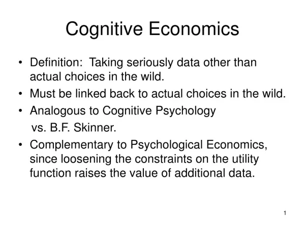
1. Cognitive Economics • Definition: Taking seriously data other than actual choices in the wild. • Must be linked back to actual choices in the wild. • Analogous to Cognitive Psychology vs. B.F. Skinner. • Complementary to Psychological Economics, since loosening the constraints on the utility function raises the value of additional data.

2. Examples of Cognitive Economics • Experimental Economics. • Neuroeconomics. • Survey measures of expectations. • Survey measures of preference parameters based on hypothetical choices. • Happiness research.

3. Labor Supply: Are the Income and Substitution Effects Both Large or Both Small? Miles Kimball and Matthew Shapiro

4. Why Study the Elasticity of Labor Supply? • Labor Economics: Labor supply elasticities are key parameters for labor economics. The existing literature is not definitive on its value. • Macroeconomics: The Frisch labor supply elasticity is a key parameter in business cycle models. Ideally, to avoid macroeconomic data-mining, it should be identified from microeconomic data. • Public Finance: The labor supply elasticity is a key parameter for public finance in determining the size of the distortions caused by labor taxation.

5. Two Slides in Honor of Ed Prescott:“Theory Ahead …” • One of the early formative experiences in my professional life was seeing Ed Prescott present “Theory Ahead of Business Cycle Measurement” at an EF meeting with Larry Summers as discussant. • Among other things, Summers criticized Prescott’s parameter values. For the labor supply elasticity, the controversial issue is that Prescott calibrates his labor supply elasticity by assuming that the marginal expenditure share of leisure is equal to the average expenditure share of leisure. • If this is not true, a direct measure of the marginal expenditure share of leisure is needed. That is what we try to provide.

6. “Why Do Americans Work So Much More Than Europeans?” • Prescott’s recent op-ed in the WSJ advertised the web link. The site was slow. • Prescott does not estimate the labor supply elasticity, but shows that if one calibrates the marginal expenditure share of leisure at 1.54/(1+1.54) = .606, differences in marginal tax rates are enough to explain why labor hours are now lower in Europe than in the U.S. and Japan. (In the early 70’s Europeans worked just as much when they faced more similar tax rates.) • Kimball and Shapiro estimate a marginal expenditure share of leisure of .581 (Table 11).

7. Areas of Agreement and Disagreement about Labor Supply • There is wide agreement that the income and substitution effects approximately cancel (i.e., that the long-run elasticity of labor supply is close to zero). • Most labor economistsbelieve the income and substitution effects are both small. • Most macroeconomistsbelieve the income and substitution effects are both large.

8. Evidence that the Long-Run Elasticity of Labor Supply ≈ 0 • Cross-National Evidence: A 10-fold difference in wages from poor to rich countries may reduces the workweek from about 44 hours to about 39 hours. • The Time Trend: A 3-fold increase in real wages has accompanied a decline in male hours and an increase in female hours, but only a modest decline in overall hours. • Cross-Sectional Evidence: Large differences in the real wage are associated with modest differences in labor hours. This is true with or without individual fixed effects.

9. Strategy of this Research • Theory: Develop a theoretical framework that imposes a zero long-run elasticity of labor supply, while allowing for • Intertemporal optimization • Integration of spousal labor supply decisions • Nonseparability between consumption and labor • Fixed cost of going to work

10. Strategy of this Research (cont.) 2. Empirics: Experimental survey approach: • Collect survey data on how a household would respond to winning a sweepstakes • Compare the change in labor hours after winning the sweepstakes to the implied change in consumption after winning the sweepstakes • Adjust for the change in job-induced consumption Ji to get the change in baseline consumption B = C – ΣJi • Frisch elasticity = -Δ ln(N)/Δ ln(B)

11. Dealing with Quits • The implication of a quit for consumption needs no adjustment • The fixed cost is calibrated to match the fact that many people work 20 hours per week, but few people work between 1 and 19 hours per week. • If someone quits, we infer that, absent the fixed cost, they would have wanted to work less than 19 hours per week. • This gives a lower bound for the labor supply elasticity of someone who quits after winning the sweepstakes.

12. Lottery Question: Suppose you won a sweepstakes that will pay you [and your (husband/wife/partner)] an amount equal to your current family income every year for as long as you [or your (husband/wife/partner)] live. We’d like to know what effect the sweepstakes money would have on your life. Would [you/your(husband/wife/partner)] Quit work entirely? If not, would you work fewer hours? If work fewer hours, how many fewer hours?

13. Overall Results: 56% Quit 21% No change 23% Reduce hours

14. Contrasting Estimates • This evidence points to a large income effect. On the assumption that income and substitution effects are equal, it also implies a large substitution effect. • When we translate that substitution effect into a Frisch elasticity and adjust for censoring, we find η=1. • By contrast, most estimates in the Labor literature for both the income and substitution effects are small, implying η<.3. • What is going on? Some clues:

15. Mulligan (1998) Finds a high Frisch elasticity in data on life-cycle intertemporal substitution by • Including older workers, who have declining wages and declining hours, (other authors exclude them because of selection worries) • Explaining the low comovement of hours and wages early in lifecycle by on-the-job training

16. Experimental and Quasi-Experimental Elasticity Estimates • Oettinger (1999): Baseball park vendors respond quite elastically to changes in effective wages from level of attendance • Farber (2003): Taxicab driver’s supply responds strongly to high-frequency variation in the implicit wage (critical of Camerer, Babcock, Loewenstein and Thaler (1997) • Fehr and Gotte (2002): Elastic behavior of bicycle messengers.

17. Imbens, Ruben and Sacerdote (2001) • Survey of state lottery winners • Individual data (decision not to collect data on spouse behavior) • Quadratic term to deal with floor of zero on labor hours • Raw MPE of .291 for the 55—65 age group, compared to .373 in our data • Lower raw MPE for younger winners, but with a substantial standard error

18. Why Does Experimental Evidence Give a Different Answer? • Institutional frictions often inhibit individual labor supply responses to small variations in the real wage or in wealth. • Experimental, quasi-experimental and experimental survey evidence involves large variations in the real wage or in wealth, or circumstances with few institutional frictions. • Exception: In negative-income tax experiments, medium-sized changes in the real wage met substantial institutional frictions that inhibited labor supply responses.

19. Econometric versus Experimental Survey Methodology • Strength of signal: • The signal for identifying the long-run elasticity of labor supply is very strong. • By contrast, the variation for identifying the income and substitution effects separately yields only a weak signal in standard data. • By construction, the experimental survey methodology involves a large amount of relevant variation and so a strong signal.

20. Econometric versus Experimental Survey Methodology (cont.) 2. Other problems with standard econometric methodology: • A small signal may get further attenuated by institutional frictions • Measurement error in wages and hours (reporting error, systematic rounding error, division biases, allocational/observed, temporary/permanent) • Endogeneity

21. Econometric versus Experimental Survey Methodology (cont.) 3. Strengths of Experimental Survey Methodology: • The shock is totally exogenous. All respondents receive the same treatment. • The shock is large enough to overcome frictions. • Robust to ordinary measurement error because only the levels of standard data figure into identification. • “Within” estimator: differences out unobserved factors like the panel approach, but no need to assume time invariance of unobserved factors.

22. Econometric versus Experimental Survey Methodology (cont.) 4. Weakness of Experimental Survey Methodology: • Response error to hypothetical questions • Survey methodology issues, such as framing, ordering and mode effects

23. Econometric versus Experimental Survey Methodology: Summary • Unlike econometric treatment of standard data, Experimental Survey Methodology can guarantee large, exogenous variation in relevant variables. • Despite the error in responses, the sampling variation in responses is a non-issue given the strong signal for 1388 workers. • Remaining issue #1: systematic biases in responses? • Remaining issue #2: theoretical interpretation of the results.

24. How Preferences and Opportunity Might Jointly Determine Outcomes • The underlying labor supply elasticity is substantial. • Over the long-run, this “deep parameter” would lead to institutional adjustments to accommodate changing hours preferences due to taxes, etc. • In the short-run, idiosyncratic changes in desired labor supply are inhibited by institutional frictions. • Because firms can coordinate work, firm-initiated changes in labor hours face weaker frictions. Thus, firms vary hours cyclically in accordance with workers’ underlying labor supply elasticities.

25. Conclusion: • Income and substitution effects approximately cancel • Hypothetical responses to large wealth shocks indicate that the income effect is large • We infer that the substitution effect is also large. • We attribute results to the contrary in the labor literature to a combination of • standard econometric problems plus • the genuine economic phenomenon of institutional frictions, which makes the response to small shocks smaller than one would expect in a frictionless world. 5. Institutional frictions imply that the large elasticities we find are relevant for some questions but not others.