Download
1 / 26
260 likes | 424 Vues
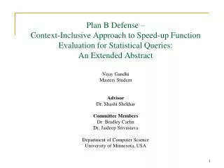
Context-Inclusive Approach to Speed-up Function Evaluation for Statistical Queries: An Extended Abstract. Vijay Gandhi, James Kang, Shashi Shekhar University of Minnesota, USA Junchang Ju, Eric D. Kolaczyk, Sucharita Gopal Boston University, USA ICDM Workshop on

E N D
Context-Inclusive Approach to Speed-up Function Evaluation for Statistical Queries: An Extended Abstract Vijay Gandhi, James Kang, Shashi Shekhar University of Minnesota, USA Junchang Ju, Eric D. Kolaczyk, Sucharita Gopal Boston University, USA ICDM Workshop on Spatial and Spatio-Temporal Data Mining December 2006
Overview • Motivation • Problem Statement • Challenges • Related Work • Contribution • Validation • Conclusion & Future Work
Motivation • Landcover Change • Loss of land - 217 square miles of Louisiana’s coastal lands were transformed to water after Hurricanes Katrina and Rita. • Deforestation – Brazil lost 150,000 sq. km. of forest between May 2000 and August 2006 • Urban Sprawl Mississippi River Delta, Louisiana (Red represents land loss between 2004 and 2005. Courtesy: USGS) Deforestation, Ariquemes, Brazil (Courtesy: Global Change Program, University of Michigan) Urban Sprawl in Atlanta (Red indicates expansion between 1976 and 1992)
Grass Conifer Hardwood Brush Land-use Class Hierarchy Likelihood of specific-classes Multiscale Multigranular Image Classification (MSMG) • Input: Class hierarchy, Likelihood of specific classes • Output: Classified images at multiple scales . . . Scale: 64x64 Scale: 4x4 Scale: 2x2 Scale: 1x1
Problem Statement • Given: • A set of hierarchical class labels • Probability densities of each specific class at (2n x 2n) pixels • Find: • Class labels for every pixel at coarser scales • Objective: • Best quality measure of each non-specific class using the function i.e., Expectation Maximization (EM) • Constraints: • Function evaluation is expensive • Coarser scales are defined implicitly in powers of 2 • 2x2, 4x4, …, 2n-1 x 2n-1
Class hierarchy C Lij(C1) Lij(C2) C1 C2 Likelihood of classes C1 and C2 at a 2x2 region Algorithm: Expectation Maximization • Given: • Class hierarchy, • Likelihood of specific classes • Find: • Best Class for a region (e.g. 2x2 region) • Likelihood of a specific class = sum of corresponding likelihood • Likelihood of non-specific class (EM): • Initialize the proportion of each corresponding specific class • Multiply each likelihood by corresponding specific class proportion • Add the likelihood at corresponding pixel • Divide the value in step 1 by corresponding value in Step 2 • Average the likelihood for each specific class • Repeat Step 2 to Step 5 until required accuracy Example
Class hierarchy C Lij(C1) Lij(C2) C1 C2 Likelihood of classes C1 and C2 at a 2x2 region Execution Trace: Expectation Maximization • Given: • Class hierarchy, • Likelihood of specific classes • Likelihood of C1 = ∑ Lij(C1)= 1.6;C2 = ∑ Lij(C2) = 1.8 • Likelihood of C: • Iteration 1: EM(p1n, p2n) • Multiply: L1ij(C1) = Lij(C1) * p1n; L2ij(C2) = Lij(C2) * p2n • Add: Lij = L1ij(C1) + L2ij(C2) • Divide: L1ij(C1) = L1ij(C1)/Lij; L2ij(C2) = L2ij(C2)/Lij • Average: p1n+1 = Avg(L1ij(C1)); p2n+1 = Avg(L2ij(C2)) EM(0.5, 0.5) • Find: Best Class for the 2x2 region 0.439, 0.560
C C1 C2 Execution Trace: Example • Computeerror = sqrt((p1n+1-p1n)2+(p2n+1-p2n)2) • if(error < Limiting Factor) • Return (p1n+1, p2n+1) • else • EM(p1n+1, p2n+1) Class hierarchy Lij(C1) Lij(C2) Limiting Factor = 0.07 0.085 > 0.07 EM(0.439,0.560) Likelihood of classes C1 and C2 at a 2x2 region • Iteration 2: EM(0.439, 0.560), error = 0.078 • Iteration 3: EM(0.3831, 0.6155), error = 0.074 • Iteration 4: EM(0.33, 0.0027), error = 0.069 • Final proportions: p1 = 0.285, p2 = 0.715 • Likelihood of C = (∑ Lij(C1)* p1 ) + (∑ Lij(C1)* p2 ) Likelihood of C1, ∑ Lij(C1) = 1.6; C2, ∑ Lij(C2) = 1.8 Likelihood of C = 0.456 + 1.286 = 1.742 • Winner = Maximum Likelihood (C, C1, C2) = C2
MSMG Classification - Formulation • Best Class at a region • = candidate models • e.g. Forest, Vegetation, Conifer • = observations • Likelihood of specific classes corresponding to M within the region • = likelihood (Quality Measure) of M • For non-specific classes, calculated using the function i.e. EM • = Penalty function • Used for non-specific classes
Related Work Multi-resolution Image Classification Other [Irons, Markham, Raptis] Formal Statistical Method Context-Exclusive [Kolaczyk et al.] Context-Inclusive
Land-use Class Hierarchy Context-Exclusive Approach • Instance Tree • Each candidate model is analyzed independently until convergence • The candidate model with maximum likelihood is selected Instance Tree 4 1. 2. 3. 4. Context-Exclusive Approach: 1. Select the best specific class, Brush 2.Vegetation is evaluated until convergence (46) 3.Forest is evaluated until convergence (34) 4.Non-Forest is evaluated until convergence (3) 5. Select the best class (Non-Forest) 1 3 2 Total iterations: 46 + 34 + 3 = 83
Limitations of Context-Exclusive Approach • Computational Scalability • For 512 x 512 pixels - 7 hours of CPU time • Where is the computational bottleneck? • 80% of total execution time is spent in computing maximum likelihood • Number of function calls is dependent on the number of pixels, and spatial scale • As spatial scale increases, • the computation time increases • exponentially CPU Time for example datasets
Land-use Class Hierarchy Contributions • Context Inclusive Approach • Instance Tree is evaluated with context • Each candidate model is analyzed until it is better than the current best • Uses a instance-level syntax tree 4 1. 2. 3. 4. 1 3 Context-Inclusive Approach: 1.Select the best specific class, Brush 2. Vegetation is evaluated until convergence (46) 3. Forest is evaluated (4) 4. Non-Forest is evaluated (1) 5. Non-Forest is the best-so-far 2 Total iterations: 46 + 4 + 1 = 51
Algorithm 2 Context-Inclusive Approach 1: Function ContextInclusive(set Cand) 2: Select the best specific class 3:for each remaining candidate model c Cand do 4:repeat 5: Refine quality measure for each candidate model c Cand 6: untilEM converges OR quality measure exceeds best so far 7: end for 8: Select candidate model that is best so far 9: return c Context-Exclusive vs. Context-Inclusive Algorithm 1 Context-Exclusive Approach 1: Function ContextExclusive(set Cand) 2: Select the best specific class 3:for each candidate model c Cand do 4:repeat 5: Refine quality measure for each candidate model c Cand 6:untilEM converges 7:end for 8: Select candidate model with the maximum quality measure 9: return c
Convergence Test • Convergence • Until ABS(Quality Measurei+1 – Quality Measurei) < Limiting Factor • Impact • As Limiting Factor decreases, Computation cost increases for Context-Exclusive • As Limiting Factor decreases, precision of Quality Measure increases for Context-Exclusive • Tradeoff • Precision of Quality Measure vs. Computation cost • Tradeoff is controlled by Limiting Factor
Experimental Design • Experimental Questions: • How does change in the limiting factor affect the Context-Exclusive approach? • How does Context-Exclusive compare to Context-Inclusive approach? • Input: Synthetic dataset and Real dataset • Language: MATLAB • Platform: UltraSparc III 1.1 GHz, 1 GB RAM • Measurements: Number of Iterations, CPU Time, Accuracy Candidates: Context-Exclusive, Context-Inclusive Classification Accuracy Measurements Compare Classifications Image Classification Benchmark Datasets Limiting Factor Experimental Design
Grass Conifer Hardwood Brush Land-use Class Hierarchy Likelihood of specific-classes Experiments – Dataset 1 • Synthetic Dataset • 128 x 128 pixels, 7 Classes • Input: Class hierarchy, Likelihood of specific classes • Output: Classified images at multiple scales . . . Scale: 64x64 Scale: 4x4 Scale: 2x2 Scale: 1x1
Experiments – Dataset 2 • Real Dataset, Plymouth County, Massachusetts • 128 x 128 pixels, 12 Classes • Input: Class hierarchy, Likelihood of specific classes … Bogs Barren Brush Pitch Pine Land-use Class Hierarchy • Output: Classified images at multiple scales . . . Scale: 1x1 Scale: 2x2 Scale: 64x64 Scale: 4x4
How does change in the Limiting Factor affect the Context-Exclusive approach? • Number of Iterations, CPU Time • Reduced the CPU time by 58% for change in limiting factor value from 0.00001 to 0.01 CPU Time Number of Iterations • Accuracy of Limiting Factor = 0.01 relative to Limiting Factor of 0.00001 • Above 99% for change in Limiting Factor to 0.01
How does Context-Exclusive Compare to Context-Inclusive? • Number of Iterations (Limiting Factor: 0.00001) • Reduced by 67% for Dataset 1 • Reduced by 61% for Dataset 2 Dataset 1 Dataset 2
How does Context-Exclusive Compare to Context-Inclusive? • Number of Iterations (Limiting Factor = 0.00001) • Reduced by 53% for Dataset 1 and 47% for Dataset 2 Dataset 1 Dataset 2 • Accuracy (Limiting Factor = 0.00001) • Above 98% for Context-Inclusive
Conclusion & Future Work • Context-Inclusive approach for function evaluation • Insight into Limiting Factor • Experimental results supporting contributions • Other methods may be explored: • Other type of context: Spatial Correlation between regions • Bottom-up strategy instead of top-down approach
Number of Iterations. Example 2 4 1. 2. 3. 4. 3 1 2 Quad: 4703, Scale: 2x2 EM Iterations Savings: 9
Number of Iterations. Example 3 4 1. 2. 3. 4. 1 3 2 Quad: 10855, Scale: 2x2 EM Iterations Savings: 19
Non-Forest Forest Vegetation Context-Exclusive Approach • Instance Tree • Each candidate model is analyzed independently until convergence • The candidate model with maximum likelihood is selected Instance Tree L3 L2 L1 Quality Measure Context-Exclusive Approach: 1.Vegetation is evaluated until convergence, L1 2.Forest is evaluated until convergence, L2 3.Non-Forest is evaluated until convergence, L3 Iterations
Non-Forest Forest Vegetation Contributions • Context Inclusive Approach • Instance Tree is evaluated with context • Each candidate model is analyzed until it is better than the current best • Uses a instance-level syntax tree L3 L2 L1 Quality Measure Context-Inclusive Approach: 1. Vegetation is evaluated until convergence, L1 2. Forest is evaluated until L2 3. Non-Forest is evaluated until L3 Iterations