INTEGRALS
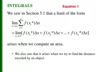
INTEGRALS. Equation 1. We saw in Section 5.1 that a limit of the form arises when we compute an area. We also saw that it arises when we try to find the distance traveled by an object. INTEGRALS.

INTEGRALS
E N D
Presentation Transcript
INTEGRALS Equation 1 • We saw in Section 5.1 that a limit of the form • arises when we compute an area. • We also saw that it arises when we try to find the distance traveled by an object.
INTEGRALS • It turns out that this same type of limit occurs in a wide variety of situations even when f is not necessarily a positive function.
INTEGRALS • In Chapters 6 and 8, we will see that limits of the form Equation 1 also arise in finding: • Lengths of curves • Volumes of solids • Centers of mass • Force due to water pressure • Work • Therefore, we give this type of limit a special name and notation.
INTEGRALS 5.2The Definite Integral
DEFINITE INTEGRAL Definition 2 • If f is a function defined for a≤ x ≤ b, we divide the interval [a, b] into n subintervals of equal width ∆x = (b – a)/n. • We let x0(= a), x1, x2, …, xn(= b) be the endpoints of these subintervals. • We let x1*, x2*,…., xn* be any sample points in these subintervals, so xi* lies in the i th subinterval.
DEFINITE INTEGRAL Definition 2 • Then, the definite integral of f from a to b is • provided that this limit exists. • If it does exist, we say f is integrable on [a, b].
DEFINITE INTEGRAL • The precise meaning of the limit that defines the integral is as follows: • For every number ε > 0 there is an integer N such that for every integer n > N and for every choice of xi* in [xi-1, xi].
INTEGRAL SIGN Note 1 • The symbol ∫was introduced by Leibniz and is called an integral sign. • It is an elongated S. • It was chosen because an integral is a limit of sums.
NOTATION Note 1 • In the notation , • f(x) is called the integrand. • a and b are called the limits of integration; a is the lower limit and b is the upper limit. • For now, the symbol dx has no meaning by itself; is all one symbol. The dx simply indicates that the independent variable is x.
DEFINITE INTEGRAL Note 2 • The procedure of calculating an integral is called integration. • The definite integral is a number. • It does not depend on x. • In fact, we could use any letter in place of x without changing the value of the integral:
RIEMANN SUM Note 3 • The sum • that occurs in Definition 2 is called a Riemann sum. • It is named after the German mathematician Bernhard Riemann (1826–1866).
RIEMANN SUM Note 3 • So, Definition 2 says that the definite integral of an integrable function can be approximated to within any desired degree of accuracy by a Riemann sum.
RIEMANN SUM Note 3 • We know that, if f happens to be positive, the Riemann sum can be interpreted as: • A sum of areas of approximating rectangles
RIEMANN SUM Note 3 • Comparing Definition 2 with the definition of area in Section 5.1, we see that the definite integral can be interpreted as: • The area under the curve y = f(x) from a to b
RIEMANN SUM Note 3 • If f takes on both positive and negative values, then the Riemann sum is: • The sum of the areas of the rectangles that lie above the x-axis and the negativesof the areas of the rectangles that lie below the x-axis • That is, the areas of the gold rectangles minusthe areas of the blue rectangles
NET AREA Note 3 • A definite integral can be interpreted as a net area, that is, a difference of areas: • A1 is the area of the region above the x-axis and below the graph of f. • A2 is the area of the region below the x-axis and above the graph of f.
UNEQUAL SUBINTERVALS Note 4 • Though we have defined by dividing [a, b] into subintervals of equal width, there are situations in which it is advantageous to work with subintervals of unequal width. • In Exercise 14 in Section 5.1, NASA provided velocity data at times that were not equally spaced. • We were still able to estimate the distance traveled.
UNEQUAL SUBINTERVALS Note 4 • There are methods for numerical integration that take advantage of unequal subintervals.
UNEQUAL SUBINTERVALS Note 4 • If the subinterval widths are ∆x1, ∆x2, …, ∆xn, we have to ensure that all these widths approach 0 in the limiting process. • This happens if the largest width, max ∆xi , approaches 0.
UNEQUAL SUBINTERVALS Note 4 • Thus, in this case, the definition of a definite integral becomes:
INTEGRABLE FUNCTIONS Note 5 • We have defined the definite integral for an integrable function. • However, not all functions are integrable.
INTEGRABLE FUNCTIONS • The following theorem shows that the most commonly occurring functions are, in fact, integrable. • It is proved in more advanced courses.
INTEGRABLE FUNCTIONS Theorem 3 • If f is continuous on [a, b], or if f has only a finite number of jump discontinuities, then f is integrable on [a, b]. • That is, the definite integral exists.
INTEGRABLE FUNCTIONS • If f is integrable on [a, b], then the limit in Definition 2 exists and gives the same value, no matter how we choose the sample points xi*. • To simplify the calculation of the integral, we often take the sample points to be right endpoints. • Then, xi* = xi and the definition of an integral simplifies as follows.
INTEGRABLE FUNCTIONS Theorem 4 • If f is integrable on [a, b], then • where
DEFINITE INTEGRAL Example 1 • Express as an integral on the interval [0, π]. • Comparing the given limit with the limit in Theorem 4, we see that they will be identical if we choose f(x) = x3 + x sin x.
DEFINITE INTEGRAL Example 1 • We are given that a = 0 and b = π. • So, by Theorem 4, we have:
DEFINITE INTEGRAL • Later, when we apply the definite integral to physical situations, it will be important to recognize limits of sums as integrals—as we did in Example 1. • When Leibniz chose the notation for an integral, he chose the ingredients as reminders of the limiting process.
DEFINITE INTEGRAL • In general, when we write • we replace: • lim Σby ∫ • xi* by x • ∆xby dx
EVALUATING INTEGRALS • When we use a limit to evaluate a definite integral, we need to know how to work with sums. • The following three equations give formulas for sums of powers of positive integers.
EVALUATING INTEGRALS Equation 5 • Equation 5 may be familiar to you from a course in algebra.
EVALUATING INTEGRALS Equation 6 and 7 • Equations 6 and 7 were discussed in Section 5.1 and are proved in Appendix E.
EVALUATING INTEGRALS Eqns. 8, 9, 10 & 11 • The remaining formulas are simple rules for working with sigma notation:
EVALUATING INTEGRALS Example 2 • Evaluate the Riemann sum for f (x) = x3 – 6x taking the sample points to be right endpoints and a = 0, b = 3, and n = 6. • Evaluate .
EVALUATING INTEGRALS Example 2a • With n = 6, • The interval width is: • The right endpoints are: x1 = 0.5, x2 = 1.0, x3 = 1.5, x4 = 2.0, x5 = 2.5, x6 = 3.0
EVALUATING INTEGRALS Example 2a • So, the Riemann sum is:
EVALUATING INTEGRALS Example 2a • Notice that f is not a positive function. • So, the Riemann sum does not represent a sum of areas of rectangles.
EVALUATING INTEGRALS Example 2a • However, it does represent the sum of the areas of the gold rectangles (above the x-axis) minus the sum of the areas of the blue rectangles (below the x-axis).
EVALUATING INTEGRALS Example 2b • With n subintervals, we have: • Thus, x0 = 0, x1 = 3/n, x2 = 6/n, x3 = 9/n. • Ingeneral, xi = 3i/n.
EVALUATING INTEGRALS Example 2b • Since we are using right endpoints, we can use Theorem 4, as follows.
EVALUATING INTEGRALS Example 2b
EVALUATING INTEGRALS Example 2b • This integral can not be interpreted as an area because f takes on both positive and negative values.
EVALUATING INTEGRALS Example 2b • However, it can be interpreted as the difference of areas A1 – A2, where A1 and A2 are as shown.
EVALUATING INTEGRALS Example 2b • This figure illustrates the calculation by showing the positive and negative terms in the right Riemann sum Rn for n = 40.
EVALUATING INTEGRALS Example 2b • The values in the table show the Riemann sums approaching the exact value of the integral, – 6.75, as n → ∞.
EVALUATING INTEGRALS • A much simpler method for evaluating the integral in Example 2 will be given in Section 5.3
EVALUATING INTEGRALS Example 3 • Set up an expression for as a limit of sums. • Use a computer algebra system (CAS) to evaluate the expression.
EVALUATING INTEGRALS Example 3a • Here, we have f (x) = ex, a = 1, b = 3, and • So, x0 = 1, x1 = 1 + 2/n, x2 = 1 + 4/n, x3 = 1 + 6/n, and xi= 1 + 2i / n
EVALUATING INTEGRALS Example 3a • From Theorem 4, we get:
EVALUATING INTEGRALS Example 3b • If we ask a CAS to evaluate the sum and simplify, we obtain: