Feasibility Of Floating-Point Arithmetic In Reconfigurable Computing Systems
230 likes | 390 Vues
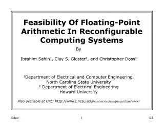
Feasibility Of Floating-Point Arithmetic In Reconfigurable Computing Systems. By Ibrahim Sahin 1 , Clay S. Gloster 2 , and Christopher Doss 1 1 Department of Electrical and Computer Engineering, North Carolina State University 2 Department of Electrical Engineering Howard University

Feasibility Of Floating-Point Arithmetic In Reconfigurable Computing Systems
E N D
Presentation Transcript
Feasibility Of Floating-Point Arithmetic In Reconfigurable Computing Systems By Ibrahim Sahin1, Clay S. Gloster2, and Christopher Doss1 1Department of Electrical and Computer Engineering, North Carolina State University 2 Department of Electrical Engineering Howard University Also available at URL: http://www2.ncsu.edu/eos/service/ece/project/rare/www/ E2
Outline of the Presentation • Introduction • Standard Floating-Point Arithmetic Modules • Example Applications • Vector Addition, Subtraction, Multiplication • Matrix Multiplication • Experimental Results for all applications • Conclusions E2
Introduction • A reconfigurable computing (RC) system is a hardware/software data processing system that combines the flexibility of a general purpose processors with the speed of application specific processors. • Several applications have been mapped onto RC systems demonstrating an order of magnitude speedup over existing solutions running on a general purpose processor. • In the past, RC systems contained very limited hardware resources. As a result, few complex applications, i.e. floating point arithmetic, could benefit from the potential speedup offered by RC systems. • Many of these complex applications were either, not • mapped to RC systems or converted to fixed-point prior to system implementation. E2
Motivation • With the recent advances in FPGA technology, including significant increases in logic capacity and clock speed, more complex applications, including those with FP arithmetic can be implemented. • Much of the RC system design methodology is manual because few tools to map high level application descriptions into hardware exist. • A C/Java compiler targeted for RC systems should be developed to reduce development time and to allow users to take advantage of the tremendous performance gains that can be achieved. • Standard modules that process assembly and machine instructions should be developed to facilitate compiler design. E2
Standard Floating-Point Module Specifications • All modules are designed to process one or more floating-point vectors. • Each module executes one or more instructions, where each instruction is a single, highly pipelined, FP vector operation. Complex applications can be developed by executing multiple instructions. • RC system memory is partitioned into two regions: instruction memory and data memory. • The instruction memory always starts from the address 0x00000. All memory following the HALT instruction is used to store input/output floating point data. E2
FPVECADD 100 200 50 Size of the vectors Start of output vector Start of input vector FPVECADDS 100 150 200 50 Size of the vectors Start of result vector Start of second vector Start of first vector A Standard Instruction Format • A module instruction includes the floating point vector operation and three or four addresses identifying the start/end of the input vector and the start of the output vector. Single Input Vector Address Instruction Two Input Vector Address Instruction • A single input vector address instruction actually operates on two vectors. However, in this case, the two vectors are interleaved. E2
FP Vector Instruction Execution • Initially one or more module configurations are loaded into the FPGA devices. • All instruction and data memory is initialized (Each FPGA has it’s own local memory.) • After initialization, all modules simultaneously begin execution. • Modules read an instruction from the instruction memory , execute the instruction, and then repeat the cycle until encountering the HALT instruction $(FFFFFF). • When the HALT instruction is reached the module stops and • sends an interrupt to the host. E2
A Standard Module Architecture • Each floating-point module consists of a standard controller, a standard datapath and a floating-point core that is instantiated in the datapath. • Using a standard controller and datapath reduces the time required to implement new modules. Standard Datapath Memory Standard Controller Controller commands Data I/O Floating-point Core Feedback signals Addr. Bus E2
Datapath Data In 32 M0 M1 CR0 CR1 CW RF Data Processor R0 R1 Fetch/Decode Unit M2 Floating-Point Core ECnt Comp. m n 32 18 4 Data Processor Micro Inst. Input Addr. Mng. Micro Inst. Input Data Out Done Final Address Out To Controller Standard Datapath • The datapath consists of two subunits, the floating point data processor and the instruction fetch/decode unit. E2
Standard Controller • The controller is implemented as a finite state machine (FSM with state transitions forming an outer and an inner loop. • At each iteration of the outer loop, an instruction is read from memory and executed. • At each iteration of the inner loop, 1-2 FP vectors are read from the memory, processed, and the result is written back to the memory. • We use micro-coded instructions in the controller to reduce design implementation and debug times. E2
Available Floating-Point Arithmetic Cores • We have completed the design and testing of three floating-point core units, adder, subtractor, and multiplier. • All FP arithmetic cores have a latency of 8 cycles. (8-stage pipeline.) • All FP arithmetic cores produce one result at every clock cycle when used in isolation. • All cores contain control circuitry that waits for data to be placed in all input registers prior to processing the data in the subsequent pipeline stages. This Distributed Control reduces the number of main controller states and simplifies the inter-core interface. E2
FP Module Integration • The core units are designed to be connected to form chains. • When both (left and right) data ready signals are active, the core begins to process the input data. • When the result is available at the output of the • core, result ready signal is asserted. Left Ready Left Data In Right Data In Right Ready 32 32 Floating Point Core 32 Result Ready Data Output E2
FP Addition, Subtraction, and Multiplication • This constitutes the first set of modules used in our research. • A single input vector address instruction processes two interleaved vectors of size k and produces a single output vector of size k. (For example, addition of 2, 64 element vectors stored in a single vector at a given address will produce a single 64 element output vector that is the sum of the two input vectors.) • All of these modules use the same datapath and main controller. Only the FP core, including it’s internal controller, is different. E2
A1 A2 B1 B2 C1 C2 D1 D2 A1 A2 B1 B2 C1 C2 D1 E D B A C D2 R/W 1 x 1 x 1 0 E D B A C E1 E2 Mem. Stages MAB MDB A B C E D E1 E2 A B C D E S1 A B C D E S2 A B C D E S3 A B C E D S4 A B C E D FP Core Unit Stages S5 A B C E D S6 A B C D E S7 S8 0 0 x 0 x 0 x 1 x 1 1 1 x x x x x x x 1 1 1 x x Memory Access: Add, Sub, Mult • The memory unit we use has a two clock cycle latency for performing a read and a one clock cycle latency for performing a write operation. • The result are written back to the memory between the read • operations. Hence, the cores produce a new element of the result every four cycles. E2
An FP Accumulator • The core includes a FP adder and a modified controller. • A single input vector accumulate instruction adds all elements of the vectors producing a single element result vector. • Replacing the adder with a subtractor, multiplier, or divider, is simple and produces novel deaccumulate, product, and division operations. E2
R/W x 0 1 1 1 1 1 Mem. Stages MAB MDB X Y Re A A B B C C D D E E F F X Y Re A X Y F B C E D S1 Y A F X B C D E S2 X A F Y B C D E S3 X F A Y B C D E S4 A X Y F B C D E FP Core Unit Stages S5 F A X Y B C E D S6 Y F X A B C D E S7 A X Y F B C D E S8 N Numbers to accumulate Emptying the accumulator Writing result 1 x 1 x x x 1 1 x x 1 1 x x 1 x Memory Access Schedule of the Accumulator Since the accumulator does not write back to memory until the end of a module instruction, it reads an element of the FP vector from the memory every clock cycle. As a result the accumulator runs almost four times as fast as the other modules. E2
Module Statistics • All modules were compiled for use in a Xilinx 4044XL device • From the table, one can conclude that approximately 5 FP adder cores or 1 FP multiplier core can fit into a single device. • Given a board with 5 of these FPGAs, 25 FP adder cores or 5 multiplier cores can be used. E2
GPP versus RC system • For a small number of FP operations, a general-purpose processor (GPP) should be faster than an RC system, but what about a large number of FP operations? • In these experiments, 131,000 FP operations were performed. (This is the maximum number of operations that can fit in 1MB of memory using our memory partitioning.) • The GPP clock speed was 300 MHz, and the FPGA board clock speed was 50 MHz. • Software versions of floating point vector addition, subtraction, and multiplication were written in C++. • Hardware versions were run on an RC system. E2
GPP versus RC System: Results *All values are in mili-second E2
PE1 Memory PE2 Memory PE1 PE2 C A B = * PE3 Memory PE4 Memory PE3 PE4 Matrix Multiplication • Matrix multiplication was selected to demonstrate how to use the FP modules to solve larger problems. • Rows of the A matrix and columns of the B matrix are • assigned to 4 processing elements (PE) or FPGA devices. E2
Matrix Multiplication (MM) • Since each PEs has 1MB memory, the largest square matrices that we can multiply is 98x98. • The matrix multiplication is performed in two sessions. In the first session, all PEs are configured with the multiplication modules and inner products are calculated. • In the final session, all PEs are configured with the accumulator to produce the results. E2
Results for Matrix Multiplication • The table above shows the module execution times in milliseconds. • Module configuration time is approximately 130 • milliseconds. • Speedup is 2-3 times over the software excluding configuration time. • To remove configuration time overhead, a future version of matrix multiplication MM can be completed in a single session using a multiply-accumulate module (MAM). E2
Conclusions • In this study we have investigated the feasibility of using FP arithmetic in RC systems and presented the results comparing the system to a general purpose processor. • CLB utilizations of the modules show that FP arithmetic operations can be used in current RC systems. • Future RC systems will only have increased FPGA resources and hence can accommodate many more FP resources. • The results showed that FP modules can achieve speedups of a factor of 5 over a typical desktop computer when 5 modules are utilized in parallel. E2