Download
1 / 50
500 likes | 669 Vues
LSST and JDEM as Complementary Probes of Dark Energy. Tony Tyson, Andy Connolly, Zeljko Ivezic, James Jee, Steve Kahn, Sam Schmidt, Don Sweeney, Dave Wittman, Hu Zhan. JDEM SCG Telecon November 25, 2008. Outline. Science drivers Hardware implementation Systematics Simulations

E N D
LSST and JDEM as Complementary Probes of Dark Energy Tony Tyson, Andy Connolly, Zeljko Ivezic, James Jee, Steve Kahn, Sam Schmidt, Don Sweeney, Dave Wittman, Hu Zhan JDEM SCG Telecon November 25, 2008
Outline • Science drivers • Hardware implementation • Systematics • Simulations • Synergy with JDEM
LSST survey of 20,000 sq deg • 4 billion galaxies with redshifts • Time domain: • 1 million supernovae • 1 million galaxy lenses • 5 million asteroids • new phenomena
LSST Survey 6-band Survey: ugrizy 320–1100 nm Frequent revisits: grizy Sky area covered: >20,000 deg2 0.2 arcsec / pixel Each 10 sq.deg field reimaged ~2000 times Limiting magnitude: 27.6 AB magnitude @5s 25 AB mag /visit = 2x15 seconds Photometry precision: 0.005 mag requirement 0.003 mag goal
Key LSST Mission: Dark Energy Precision measurements of all dark energy signatures in a single data set. Separately measure geometry and growth of dark matter structure vs cosmic time. • Weak gravitational lensing correlations (multiple lensing probes!) • Baryon acoustic oscillations (BAO) • Counts of dark matter clusters • Supernovae to redshift 0.8 (complementary to JDEM) • Probe anisotropy
deep wide fast: 320 sq.m sq.deg
LSST six color system Includes sensor QE, atmospheric attenuation, optical transmission functions Relative system throughput (%) Wavelength (nm)
2d Focal plane Sci CCD 40 mm The LSST Focal Plane Guide Sensors (8 locations) Wavefront Sensors (4 locations) Wavefront Sensor Layout Curvature Sensor Side View Configuration 3.5 degree Field of View (634 mm diameter)
I1 I2 WCS processing: get the perturbation wavefronts Get intra and extra focal image intensities. * Tools used for simulations and calculations: Zemax Matlab LSST reconstruction pipeline simulator Perturbations Get correction vector by solving Normal equation. (A: sensitive matrix, f0: error vector.)
Active optics Correct for perturbations due to thermal and mechanical distortions Each optic has 6 dof (decenter, defocus, three euler angles) Perturbations are placed on the three mirrors using a Zernike expansion to simulate the possible residual control system errors each mirror can have an arbitrary amplitude code goes up to 5th order polynomials e.g. Mirror Defocus Perturbation spectrum
FWHM Allocation & Budget meets SRD Requirements Margin available No Explicit Camera Allocation For Thermal Effects Some Telescope Thermal Effects Included
The LSST CCD Sensor 16 segments/CCD200 CCDs total3200 Total Outputs
The LSST site in Chile photometric calibration telescope
Brookhaven National Laboratory California Institute of Technology Carnegie Mellon University Columbia University Google Inc. Harvard-Smithsonian Center for Astrophysics Johns Hopkins University Las Cumbres Observatory Lawrence Livermore National Laboratory National Optical Astronomy Observatory Princeton University Purdue University Research Corporation Rutgers University Stanford Linear Accelerator Center Stanford University –KIPAC The Pennsylvania State University University of Arizona University of California, Davis University of California, Irvine University of Illinois at Champaign-Urbana University of Pennsylvania University of Pittsburgh University of Washington There are 24 LSSTC US Institutional Members No proprietary time + IN2P3 in France Funding: Public-Private Partnership NSF, DOE, Private
Figure : Visits numbers per field for the 10 year simulated survey LSST imaging & operations simulations Sheared HDF raytraced + perturbation + atmosphere + wind + optics + pixel LSST Operations, including real weather data: coverage + depth Performance verification using Subaru imaging
10-year simulation: limiting magnitudes per 30s visit in main survey1 visit = 2 x 15 sec exposures Opsim5.72 Nov 2008
10-year simulation: number of visits per band in main survey Opsim5.72 Nov 2008
LSST and Cosmic Shear Ten redshift bins yield 55 auto and cross spectra useful range baryons + higher order
LSST Precision on Dark Energy [in DETF language] Combining techniques breaks degeneracies. Joint analysis of WL & BAO is less affected by the systematics
Critical Issues • WL shear reconstruction errors • Show control to better than required precision using existing new facilities • Photometric redshift errors • Develop robust photo-z calibration plan • Undertake world campaign for spectroscopy () • Photometry errors • Develop and test precision flux calibration technique
Residual shear correlation Test of shear systematics: Use faint stars as proxies for galaxies, and calculate the shear-shear correlation after correcting for PSF ellipticity via a different set of stars. Compare with expected cosmic shear signal. Conclusion: 200 exposures per sky patch will yield negligible PSF induced shear systematics. Wittman (2005) Cosmic shear signal Stars
LSST: Gold sample: 4 billion galaxies i<25 (S/N=25), out of 10 billion detected. 56/sq.arcmin ~40 galaxies per sq.arcmin used for WL HST ACS data
residual galaxy shear correlation Single 10 sq.deg field full depth Galaxy residual shear error is shape shot noise dominated. Averages down like 1/N fields to the systematic floor. Survey of 20,000 sq.deg will have N ~ 2000 fields in each red band r, i, z Simulation of 0.6” seeing. J. Jee 2008
IMAGE SIMULATIONS All Sky Database Milkyway Extended Sources Transients Defects Base Catalog Solar System Cosmology Generate the seed catalog as required for simulation. Includes: Instance Catalog Generation Operation Simulation Metadata Size Position Color Brightness Proper motion Type Variability DM Data base load simulation Source Image Generation Introduce shear parameter from cosmology metadata Generate per FOV Atmosphere Photon Propagation Operation Simulation Telescope Camera Defects Generate per Sensor Formatting DM Pipelines Calibration Simulation LSST Sample Images and Catalogs
Input catalog for simulations 32 • Millennium Simulations Kitzbichler and White (2006) • 6 fields, 1.4x1.4 deg per field • 6x10⁶ source per catalog • Based on Croton et al (2006) and De Lucia and Blaizot (2006) models • r<26 magnitude limit • z<4 redshift limit • BVRIK Johnson and griz SDSS • Estimated u and y passbands • Type and size included
Photo-z Simulations Abdalla etal. 2008 J=23.4 10 sigma
Calibrating photometric redshifts Cross-correlation LSS-based techniques can reconstruct the true z distribution of a photo-z bin, even with spectroscopy of only the brightest galaxies at each z. These techniques meet LSST requirements with easily attainable spectroscopic samples, ~104 galaxies per unit z. Newman 2008
multiple probes of dark energy • WL shear-shear tomography • WL bi-spectrum tomography • Distribution of 250,000 shear peaks • Baryon acoustic oscillations • 1 million SNe Ia, z<1 per year • Low l, 2p sky coverage: anisotropy? • 3x10⁹ galaxies, 106 SNe • probe growth(z) and d(z) separately • multiply lensed AGNs and SNe
JDEM-LSST Complementarity • JDEM+LSST in 20,000 sq.deg and in fifty 10 sq.deg deep drilling fields • Estimated cosmological constraints using LSST+JDEM • Optimum strategy for joint DE mission risk reduction • Priorities for max complementarity and cost effectiveness
JDEM-LSST Priorities • Two IR bands from space. Deep, wide. Helps photo-z plus lots of astronomy (galaxy evolution, stellar) • JDEM spectroscopic BAO complements LSST 2-D BAO • JDEM coverage of same 20,000 sq.deg (see #1) • Four near IR bands from space, closing the zY gap • JDEM WL coverage of some of LSST’s survey area Need quantitative modeling for joint design mission. It will be useful to simulate the increase in FoM for each priority
Requirement of integrated 50 galaxies per sq.arcminute: green line in the following plot. The corresponding 10 sigma limiting magnitudes in r and i are: r=25.6 i=25.0 AB mag
WL shear power spectrum and statistical errors Signal LSST: fsky = 0.5, ng = 40 SNAP: fsky = 0.1, ng =100 RMS intrinsic contribution to the shear σg= 0.25 (conservative). No systematics! Jain, Jarvis, and Bernstein 2006 Noise SNAP LSST gastrophysics
Trade with depth and systematics LSST only
Galaxy ellipticity systematics in the SRD Specification: The median LSST image (two per visit) must have the median E1, E2, and Ex averaged over the FOV, less than SE3 for 1 arcmin, and less than SE4 for 5 arcmin. No more than EF2 % of images will exceed values of SE5 for 1 arcmin, nor SE6 for 5 arcmin
DETF FoM vs Etendue-Time Separate DE Probes Combined JDEM+LSST will be even better