Neural Network Model Optimization for Movie Ratings Prediction
Sue seeks to enhance movie rating predictions with a neural network model. Explore learning algorithms and bagging for improved predictions.

Neural Network Model Optimization for Movie Ratings Prediction
E N D
Presentation Transcript
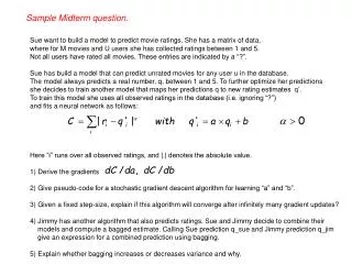
Sample Midterm question. Sue want to build a model to predict movie ratings. She has a matrix of data, where for M movies and U users she has collected ratings between 1 and 5. Not all users have rated all movies. These entries are indicated by a “?”. Sue has build a model that can predict unrated movies for any user u in the database. The model always predicts a real number, q, between 1 and 5. To further optimize her predictions she decides to train another model that maps her predictions q to new rating estimates q’. To train this model she uses all observed ratings in the database (i.e. ignoring “?”) and fits a neural network as follows: Here “i” runs over all observed ratings, and |.| denotes the absolute value. 1) Derive the gradients 2) Give pseudo-code for a stochastic gradient descent algorithm for learning “a” and “b”. 3) Given a fixed step-size, explain if this algorithm will converge after infinitely many gradient updates? 4) Jimmy has another algorithm that also predicts ratings. Sue and Jimmy decide to combine their models and compute a bagged estimate. Calling Sue prediction q_sue and Jimmy prediction q_jim give an expression for a combined prediction using bagging. 5) Explain whether bagging increases or decreases variance and why.
Bayesian Learning Instructor: Max Welling Read chapter 6 in book.
Probabilities • Building models with probability distributions is important because: • We can naturally include prior knowledge • We can naturally encode uncertainty • We can build models that are naturally protected against overfitting. • We define multivariate probability distributions over discrete sample spaces by • Probability densities are different beasts. They are defined over continuous • sample spaces and we have Can P(x) > 1 for probability densities? How about discrete distributions?
Conditional Distributions • A conditional distribution expresses the remaining uncertainty in x, • after we know the value for y. • Bayes rule: • Useful for assessing diagnostic probability from causal probability: • P(Cause|Effect) = P(Effect|Cause) P(Cause) / P(Effect) • E.g., let M be meningitis, S be stiff neck: P(m|s) = P(s|m) P(m) / P(s) = 0.8 × 0.0001 / 0.1 = 0.0008 • Note1: even though the probability of having a stiff neck given meningitis is very large (0.8), the posterior probability of meningitis given a stiff neck is still very small (why?). • Note2: P(s|m) only depends on meningitis (a stable fact), but P(m|s) depends on whether e.g. the flu is around.
(Conditional) Independence • There are two equivalent ways you can test for independence between two • random variables. • Conditional independence is a very powerful modeling assumption. It says: • Note that this does not mean that P(x,y)=P(x)P(y). Only x and y are only • independent given a third variable.
smog lung cancer asthma Example C.I. • Asthma and lung cancer are not • independent (more people with asthma • also suffer from lung cancer). • However, there is a third cause, that • explains why: smog causes both asthma • and lung-cancer. • Given that we know the presence of • smog, asthma and lung-cancer become • independent. • This type of independency can be • graphically using a graphical model.
Bayesian Networks smog • To every graphical model corresponds • a probability distribution. • More generally: • To every graphical model corresponds a list • of (conditional) independency relations that • we can either read off from the graph, or prove • using the corresponding expression. • In this example we have: • This implies marginal independence between • Eq and Ct: lung cancer asthma earth quake cat enters house alarm Prove this
earth quake cat enters house alarm Explaining Away • If we don’t know whether the alarm went off, Eq and Ct are independent. • If we observe “alarm goes off” are Eq and Ct still independent in this case? • Answer: no! • So, the alarm went off. Since earthquakes are very unlikely, you thought it • must have been the cat again touching the alarm: • However, now you observe the cat was with friends (you now observe • information about Ct). Do you now think an earthquake was more likely? • (note: Alarms can also go off at random)
class label attribute 4 attribute 5 attribute 2 attribute 3 attribute 1 Naive Bayes Classifier attribute 1
NB Classifier • First we learn the conditional probabilities • and (later) • To classify we use Bayes rule and maximize over y • We can equivalently solve:
Multinomial Distribution • For count data the multinomial distribution is often appropriate. • Example: a,a,b,a,b,c,b,a,a,b with: • The probability of this particular sequence is: Q=0.6x0.6x0.3x0.6x0.3x0.1x0.3x0.6x0.6x0.3 • The probability of a sequence with 5 a’s, 4 b’s and 1 c is: 10!/5!4!1! x Q • Longer sequences are have less prob. because there are more of them and:
Example: Text • Data consists of documents from a certain class y. • Xi is a count of the number times words “i” is present in the document. • We can imagine that we throw all words in a certain class on one big pile • and forget about the particular document it came from (it’s like a very long doc.) • We use multinomials, but “forget” about the counting factor (it doesn’t matter). • Every word can be thought of as a sample from the multinomial. • We describe the probability that a word in a document in class y is equal to • vocabulary word “i” to be: • Also, the probability that a document is from class c is given by: • The probability of a document is (in a given word order): • So, classification for a new test document (with unknown c) boils down to:
Learning NB • One can maximize the log-probability of the data under the model: • Taking derivatives and imposing the normalization constraints, one finds: • So learning is really easy: It’s just counting!
Smoothing • With a large vocabulary, there may not be enough documents in class c to have • every word in the data. E.g. the word mouse was not encountered in documents • on computers. • This means that when we happen to encounter a test document on computers • that mentions the word mouse, the probability of it belonging to the class • computers is 0. • This is precisely over-fitting (with more data this would not have happened). • Solution: smoothing (Laplace correction): # of imaginary extra docs smooth a priory estimate of # of imaginary extra words in class c smooth a priory estimate of
Document Clustering • In the NB classifier, we knew the class-label for each document • (supervised learning). What if we don’t know the class label? Can we • find plausible class-labels? (clustering / unsupervised learning). • This is precisely the same as mixtures of Gaussians. But this time we replace • Gaussians with discrete probabilities • The algorithm again alternates 2 phases: • M-step: Given cluster assignments (labels), update parameters as in NB. • E-step: infer plausible cluster labels given your current parameters. “hard” E-step “hard” M-step
Soft Assignment Clustering • We can generalize these equations to soft-assignments “soft” E-step “soft” M-step
Semi-Supervised Learning • Now imagine that for a small subset of the data you know • the labels, but for the remainder you don’t. • This is the general setup for semi-supervised learning. • The EM algorithm from the previous slides is very well • suited to deal with this problem. • Run soft E and M steps, but whenever you happen to know • the label for document “doc”, use: • This sets is just a mix between NB and clustering. • Caution: Local minima are sometimes problematic.
Bayesian Networks • If all variables are observed • learning just boils down to counting • Sometimes variables are never observed. • This are called “hidden” or “latent” variables. • Learning is now a lot harder, because • plausible fill-in values for these variables • need to be inferred. • BNs are very powerful expert systems.
Full Bayesian Approaches • The idea is to not fit anything (so you can’t over-fit). • Instead we consider our parameters as random variables. • If we place a prior distribution on the parameters, we can simply • integrate them out (now they are gone!). • Remember though that bad priors lead to bad models, it’s not a silver bullet. • In the limit of large numbers of data-items, one can derive the MDL penalty: • Computational overhead for full Bayesian approaches can be large.
Conclusions • Bayesian learning is learning with probabilities and using Bayes rule. • Full Bayesian “learning” marginalizes out parameters • Naive Bayes models are “generative models” in that you imagine how data • is generated and then invert it using Bayes rule to classify new data. • Separate model are trained for each class! • All other classifiers seen so far are discriminative. Decision surface were • trained on all classes jointly. With many data-items discriminative is expected • to better, but for small datasets generative (NB) is better. • When we don’t know the class label y in NB, we have a hidden variable. • Clustering is like fitting a NB model with hidden class label. MoG uses • Gaussian conditional distributions. If we use discrete distributions (q) we are • fitting a “mixture of multinomials”. This is a good model to cluster text documents.