Variations in stock prices appear to have a strong random component.

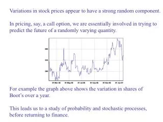
1. Variations in stock prices appear to have a strong random component. In pricing, say, a call option, we are essentially involved in trying to predict the future of a randomly varying quantity. For example the graph above shows the variation in shares of Boot’s over a year. This leads us to a study of probability and stochastic processes, before returning to finance.

2. We adopt a fairly intuitive rather than an axiomatic approach. Suppose we have some experiment which can give rise to a number of possible results - eg drawing a card from a pack. Each performance of the experiment is called a trial, and each possible result an outcome. So, if we draw a card , the possible outcomes are the 52 cards which we may draw. The set of outcomes is called the sample space. Often we may not be interested in individual outcomes, but in whether the outcome belongs to some subset of the sample space. Such subsets are called events.

3. Possible events • Draw a club • Draw a ten • Draw a face card Note that events need not be mutually exclusive.

4. Now, we introduce the probability of an event A as the relative • frequency with which it will occur in a large number of trials. • So • P(Drawing an ace)=1/13 • P( Drawing the ace of spades)=1/52 From this definition it is clear that for any event A If S is the entire sample space, then This says that we must get one of the possible outcomes.

5. If is the complement of A, ie the set of outcomes not in A, then If A and B two events, then The union means that either event occurs and the intersection that both events occur. When we add the probability of A to that of B the intersection is counted twice. Let A be the event that we draw a club, B that we draw an ace. Then P(Club or Ace)=P(Club)+P(Ace)-P(Ace of clubs) =1/4 +1/13-1/52

6. Conditional Probability. P(A|B)=Probability of A given that B has occurred. We have The first of these says that the probability of A and B is the probability of B given A times the probability that A occurs in the first place. A and B are statistically independent if P(A|B)=P(A) ie if the probability of A is independent of whether B occurs or not. For such events

7. Random Variables Suppose that each of the possible outcomes from a sample space S has a real number X associated with it.. Then X is called a random variable. If a probability can be assigned to each outcome then a probability distribution can be assigned to any random variable. Random variables can be discrete or continuous, Discrete random variable takes values x1, x2 …… xn , ie a finite (or at most countable set) - eg, number of heads in 10 throws of a coin. Continuous random variable can take any value on the real line or on some interval of the real line - eg height of an individual, price of a share.

8. If X is a discrete random variable, we can assign a probability to each value. The sum of these probabilities has to be 1. For a continuous variable we define the probability density function (PDF) to be such that the probability that X lies in a small interval between x and x+dx is f(x)dx. The PDF has to be a real function which is everywhere positive. Also, the fact that the sum of probabilities over all possible outcomes is 1 translates to If the value of X is confined to some subset of the real numbers, the range of the integral can be adjusted accordingly.

9. It is sometimes useful to introduce a cumulative probability function F(x) such that F(x) is the probability that X≤x . Then and

10. If g(X) is some function of the random variable, then the expectation value of g(X) is for a continuous distribution. For a discrete distribution where Pi is the probability if the value xi,

11. The mean of a distribution is the expectation value of X itself, E[X]. Generally it is denoted by  It is just the average value of X that we would expect to find over a large number of trials. The variance of a distribution is and its standard deviation is The SD is a measure of the spread of the values of X around the mean.

12. We now turn to some important distributions which occur in practice. Binomial distribution. Suppose that each trial has two possible outcomes (like tossing a coin). Call one a success, and let it occur with probability p, and the other a failure, occurring with probability 1-p. Let X be the random variable defined by the number of successes in n trials. This is a discrete random variable which can take values from 0 to n. The probability of obtaining some particular sequence with x successes and n-x failures is and the number of sequences of this sort is the binomial coefficient

13. So, the probability of obtaining x successes, regardless of the order in which they occur, is This is the binomial probability distribution. If the random variable X follows the binomial distribution for n trials with probability of success p, we write

14. The following slide shows a binomial distribtion. p=0.6 Number of trials=8

16. The most important continuous distribution is the Gaussian distribution or Normal distribution of the form From the result it can be seen that this is a properly normalised distribution with mean and SD 

17. Since the effect of changing and is just to shift the origin of the distribution it is often convenient to deal with a standard Gaussian where and  In a Gaussian distribution, approximately 2/3 of values lie within one standard deviation of the mean, about 95% within two standard deviations and 99.75 within three standard deviations. The next page shows a graph of the standard Gaussian.

19. The Central Limit Theorem states that if Xi , I=1…n are independent random variables described by distribution functions with mean iand SD ithen the random variable has the following properties. Its expectation value is the average of the I ‘s. Its variance is Its distribution tends to a Gaussian as n becomes large. This holds regardless of the form of the individual distributions, which need not all be of the same form. All they need is finite mean and SD.

20. The Central Limit Theorem explains the importance of Gaussian distributions. Any process which is the result of a large number of separate events will tend to produce a Gaussian. For example, Brownian motion is the random motion of small particles in a fluid, resulting from collisions with molecules in the fluid. Over any macroscopic time interval the deflection is the result of many collisions and is distributed according to a Gaussian.

21. The next slide shows a histogram of 100,000 numbers chosen randomly from the interval [0,1]. This interval was divided into 100 equal parts and the number of values in each subinterval plotted. Each number is around 1,000 as expected.

23. Now, the same set of data is taken in groups of 10 and the average of each such group calculated. The distribution of these 10,000 averages over the same 100 subintervals of [0,1] is then plotted. The shape is now a fair approximation to Gaussian.