Understanding Quantum Experiment: Computing Probabilities
Exploring a simple quantum experiment that computes probabilities in a sensible way. Discusses the square roots of probability and complex amplitudes. A deep dive into photon polarization and communication puzzles.

Understanding Quantum Experiment: Computing Probabilities
E N D
Presentation Transcript
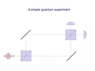
Computing probabilities in a sensible way (½)(½)+(½)(½) = ½ ½ ½
The experimental result 0% 100%
Questions Why do we have to work with “square roots” of probability? Is there a deeper explanation? And why are these “square roots” complex? I will try to answer the first question—why square roots? But my answer will make the second question worse. Then I address the second question—why complex amplitudes?—and ask in particular whether the real-amplitude theory could conceivably be correct.
Photon polarization polarizing filter
Measuring photon polarization polarizing filter
Measuring photon polarization 42° polarizing filter
Measuring photon polarization 42° polarizing filter There is no such device.
Measuring photon polarization polarizing beam splitter polarizing filter
Measuring photon polarization polarizing beam splitter polarizing filter
Measuring photon polarization By measuring many photons, we can estimate the probability of the vertical outcome. This tells us about the angle. polarizing filter
The standard account of probability vs angle Squaring the amplitude gives the probability: p q amplitude for vertical q
A completely different explanation for that curve: Optimal information transfer? The angle varies continuously. But the measurement is probabilistic with only two possible outcomes. Is the communication optimal? polarizing filter
A Communication Puzzle q Alice is going to think of a number q between 0 and p/2.
A Communication Puzzle q Alice is going to think of a number q between 0 and p/2. She will construct a coin, with her number encoded in the probability of heads.
A Communication Puzzle q Alice is going to think of a number q between 0 and p/2. She will construct a coin, with her number encoded in the probability of heads. She will send the coin to Bob.
A Communication Puzzle q Alice is going to think of a number q between 0 and p/2. She will construct a coin, with her number encoded in the probability of heads. She will send the coin to Bob. To find q, Bob will flip the coin...
A Communication Puzzle q Alice is going to think of a number q between 0 and p/2. She will construct a coin, with her number encoded in the probability of heads. She will send the coin to Bob. To find q, Bob will flip the coin, but it self-destructs after one flip.
The Goal: Find the optimal encoding p(q) q Maximize the mutual information: Here n is the number of heads Bob tosses (n = 0 or 1), and q is distributed uniformly between 0 and p/2.
An Optimal Encoding (1 flip) (Information-maximizing for a uniform a priori distribution.) 1 probability of heads 0 0 p/2 Alice’s number q
Modified Puzzle—Bob Gets Two Flips q The coin self-destructs after two flips. (It’s like sending two photons with the same polarization.)
An Optimal Encoding (2 flips) 1 probability of heads 0 0 p/2 Alice’s number q
New Modification—Bob Gets 25 Flips q The coin self-destructs after 25 flips. (It’s like sending 25 photons with the same polarization.)
An Optimal Encoding (25 flips) 1 probability of heads 0 0 p/2 Alice’s number q
Taking the limit of an infinite number of flips For any given encoding pheads(q), consider the following limit. We ask what encodings maximize this limit.
An optimal encoding in the limit of infinitely many flips 1 probability of heads 0 0 p/2 Alice’s number q This is exactly what photons do!
Why this works: Wider deviation matches greater slope 1 n/N N = number of tosses. n/N 0 p/2 0 Alice’s number
Another way of seeing the same thing Δ(n/N) pictured on the probability interval. 1 1 same size p2 p2 0 0 p1 1 0 1 0 p1 Using square roots of probability equalizes the spread in the binomial distribution.
A Good Story In quantum theory, it’s impossible to have a perfect correspondence between past and future (in measurement). But the correspondence is as close as possible, given the limitations of a probabilistic theory with discrete outcomes. This fact might begin to explain why we have to use “square roots of probability.”
But this good story is not true! Why not?
But this good story is not true! Why not? Because probability amplitudes are complex.
No information maximization in the complex theory. | An orthogonal measurement completely misses a whole degree of freedom (phase). | | pvertical= cos2(/2), but is not uniformly distributed. |
Quantum theory with d orthogonal states: With real amplitudes, information transfer is again optimal. p3 a3 a2 p2 a1 p1 The rule pkak2 again maximizes the information gained about a, compared with other conceivable probability rules, in the limit of an infinite number of trials.
Making statistical fluctuations uniform and isotropic p3 p3 p2 p2 p1 p1 In this sense real square roots of probability arise naturally.
But again, information transfer is not optimal in standard quantum theory with complex amplitudes. Inddimensions, a pure state holds 2(d1) real parameters, but there are only d1 independent probabilities for a complete orthogonal measurement. Why complex? Why this factor of 2?
Conceivable answers to “Why complex amplitudes?” Want an uncertainty principle (Stueckelberg; Lahti & Maczynski) Want local tomography (Hardy; Chiribellaet al; Müller & Masaneset al; Dakić & Brukner; me) Want complementarity(Goyalet al) Want square roots of transformations (Aaronson) Want algebraic closure (many people)
A Different Approach: Maybe the real-amplitude theory is correct. Require that every real operator commute with where Then the real theory in 2d dimensions becomes equivalent to the complex theory in d dimensions.
Our take on Stueckelberg’s idea: The ubit model (with AntoniyaAleksandrova and Victoria Borish) • Assume: • Real-amplitude quantum theory • A special universal rebit (ubit)—doubles the dimension • The ubit interacts with everything ubit local system environment We can get an effective theory similar to standard quantum theory.
Roughly, the ubit plays the role of the phase factor. The ubit’s state space: |i -|1 |1 But treating it as an actual physical system makes a difference. -|i
ubit The dynamics local system A environment E Generated by an antisymmetric operator S: • w is the ubit’s rotation rate. • s is the strength of the ubit-environment interaction. • BEU is chosen randomly. • We do perturbation theory, with s/w as our small parameter.
ubit Effect of the environment on the ubit The state of UA has components proportional to JU and XU and ZU. local system A environment E coefficient of JU coefficient of XU time time We assume (i) rapid rotation of the ubit and (ii) strong interaction with the environment, so that the above processes happen much faster than any local process.
What we assume in our analysis: • Both s (ubit-environment interaction strength) and w (ubit • rotation rate) approach infinity with a fixed ratio. • Infinite-dimensional state space of the environment; • thus, infinitely many random parameters in BEU. • What we find for the effective theory of the UA system: • We recover Stueckelberg’s rule: all operators commute • with JU. • There is no signaling through the ubit (for a UAB system). • As s/w approaches zero, we seem to recover standard • quantum theory. • Short of this limit, we see deviations from the standard • theory. We see three distinct effects:
z Precessingqubit x (i) Retardation of the evolution (second order in s/w) x component of Bloch vector s/w = 0.3 time
z Precessingqubit x (i) Retardation of the evolution (second order in s/w) x component of Bloch vector Not sure how to look for this effect. There’s another special axis that is not special in standard quantum theory. time
z Precessingqubit x (ii) Flattening of the Bloch sphere (second order in s/w) x component of Bloch vector s/w = 0.1 time