Download
1 / 13
130 likes | 271 Vues
Archive To Ecogrid. Registered Ecogrid Database. Registered Ecogrid Database. Registered Ecogrid Database. Registered Ecogrid Database. Test sample (d). DiGIR Species presence & absence points (a). Native range prediction map (f). Training sample (d). GARP rule set (e).

E N D
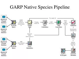
Archive To Ecogrid Registered Ecogrid Database Registered Ecogrid Database Registered Ecogrid Database Registered Ecogrid Database Test sample (d) DiGIR Species presence & absence points (a) Native range prediction map (f) Training sample (d) GARP rule set (e) Data Calculation Map Generation EcoGrid Query EcoGrid Query Validation User Sample Data +A2 +A3 Generate Metadata Layer Integration Model quality parameter (g) +A1 Integrated layers (native range) (c) SRB Environmental layers (b) Selected prediction maps (h) GARP Native Species Pipeline
Archive To Ecogrid Test sample j (d) Registered Ecogrid Database Registered Ecogrid Database Registered Ecogrid Database Registered Ecogrid Database Training sample not j (d) GARP rule set (e) When j = i DiGIR Species presence & absence points (a) Data Calculation (GARP) Data Calculation (GARP) Map Generation EcoGrid Query EcoGrid Query Validation User Model quality parameters (g) Data Integration Sample Data For j = 1 to i +A2 +A3 +A3 +A2 Native range prediction map (f) Generate Metadata Layer Integration Training data (d) GARP rule set (e) +A1 +A1 Selected prediction maps (h) Integrated layers (native range) (c) SRB Environmental layers (b) GARP with Validation Pipeline
Archive To Ecogrid Registered Ecogrid Database Registered Ecogrid Database Registered Ecogrid Database Registered Ecogrid Database Data Calculation Map Generation EcoGrid Query EcoGrid Query User Validation Subset Samples (i) sets Sample Data +A3 +A2 +A3 +A2 Generate Metadata Layer Integration +A1 +A1 GARP/Cross Validation Pipeline Test sample j (f) DiGIR Species presence & absence points (a) Training sample not j (e) GARP rule set (g) Sample set (d) For j = 1 to i Model validation matrix (h) Integrated layers (native range) (c) Selected model (i) SRB Environmental layers (b) Native range prediction map (j)
Registered Ecogrid Database Registered Ecogrid Database Registered Ecogrid Database Registered Ecogrid Database (d) Sample Data (a) Data Calculation (d) (e) (f) EcoGrid Query Map Generation Validation +A2 +A3 (g) (c) +A1 Archive To Ecogrid Generate Metadata EcoGrid Query Layer Integration (b) User (h) GARP Native Species Pipeline B&W
Species distribution caption Figure _. Modeling the distribution of a species using appropriate ecological niche modeling algorithms (e.g., GARP—the Genetic Algorithm for Rule-set Production) in an analytical pipeline environment. a) The EcoGrid is queried for data specifying the presence or absence of a particular species in a given area. b) Multiple environmental layers relevant to the specie’s distribution are selected with a second EcoGrid query. c) Environmental layers are spatially- integrated into layer stacks. d) Samples are selected from the presence/absence data, and the corresponding values from the environmental layer stack are retrieved. The sample is divided into a training set and a testing set. e) The GARP algorithm is run on the training set. The GARP ruleset is then applied to the entire area, creating a predictive map. f) Predictive maps are sent to the scientist’s workstation for further analysis. g) A comparison is made between the ground truth occurrence data that were set aside as test data, and the corresponding location on the predictive map. Error measures providing an indication of model quality are sent to the scientist’s workstation. h) After multiple runs, the user may select maps for metadata generation and archiving back to the EcoGrid.
Archive To Ecogrid Registered Ecogrid Database Registered Ecogrid Database Registered Ecogrid Database Registered Ecogrid Database Test sample (d) Species presence & absence points (native range) (a) Native range prediction map (f) Training sample (d) GARP rule set (e) Data Calculation Map Generation Map Generation EcoGrid Query EcoGrid Query User Validation Sample Data Model quality parameter (g) +A3 +A2 Integrated layers (native range) (c) Generate Metadata Layer Integration Layer Integration Environmental layers (native range) (b) +A1 Climate change prediction map (f) Selected prediction maps (h) Environmental layers (changed range) (b) Integrated layers (changed range) (c) GARP Climate Change Pipeline
Registered Ecogrid Database Registered Ecogrid Database Registered Ecogrid Database Registered Ecogrid Database Test sample (d) Sample Data Data Calculation EcoGrid Query (a) (d) (e) Map Generation (f) Validation +A2 +A3 (g) (c) +A1 (b) (h) Archive To Ecogrid Generate Metadata Layer Integration User (f) (b) (c) EcoGrid Query Layer Integration Map Generation GARP Climate Change Pipeline B&W
Climate change caption Figure _. Modeling the distribution of a species using appropriate ecological niche modeling algorithms (e.g., GARP—the Genetic Algorithm for Rule-set Production) in an analytical pipeline environment. a) The EcoGrid is queried for data specifying the presence or absence of a particular species in a given area. b) Multiple environmental layers relevant to the specie’s distribution are selected with a second EcoGrid query. c) Environmental layers, representing current conditions and potential conditions after climate change, are spatially- integrated into layer stacks. d) Samples are selected from the presence/absence data, and the corresponding values from the environmental layer stack are retrieved. The sample is divided into a training set and a testing set. e) The GARP algorithm is run on the training set. The GARP ruleset is then applied to the entire area, creating predictive maps under current conditions (native range) and after climate change (changed range). f) Predictive maps are sent to the scientist’s workstation for further analysis. g) A comparison is made between the ground truth occurrence data that were set aside as test data, and the corresponding location on the predictive map of current conditions. Error measures providing an indication of model quality are sent to the scientist’s workstation. h) After multiple runs, the user may select maps for metadata generation and archiving back to the EcoGrid.
Archive To Ecogrid Registered Ecogrid Database Registered Ecogrid Database Registered Ecogrid Database Registered Ecogrid Database Test sample (d) Species presence & absence points (native range) (a) Native range prediction map (f) Training sample (d) GARP rule set (e) Data Calculation Map Generation Map Generation EcoGrid Query EcoGrid Query User Validation Validation Sample Data +A2 +A3 Model quality parameter (g) Generate Metadata Integrated layers (native range) (c) Layer Integration Layer Integration +A1 Environmental layers (native range) (b) Invasion area prediction map (f) Selected prediction maps (h) Model quality parameter (g) Integrated layers (invasion area) (c) Environmental layers (invasion area) (b) Species presence &absence points (invasion area) (a) GARP Invasive Species Pipeline
(a) Registered Ecogrid Database Registered Ecogrid Database Registered Ecogrid Database Registered Ecogrid Database (d) Data Calculation (a) (d) (e) EcoGrid Query (f) Validation +A2 +A3 Map Generation Sample Data (g) (c) +A1 (b) (h) Archive To Ecogrid Generate Metadata Layer Integration User (g) (b) (c) (f) Map Generation EcoGrid Query Layer Integration Validation GARP Invasive Species Pipeline B&W
Invasive species caption Figure _. Modeling the distribution of a species using appropriate ecological niche modeling algorithms (e.g., GARP—the Genetic Algorithm for Rule-set Production) in an analytical pipeline environment. a) The EcoGrid is queried for data specifying the presence or absence of a particular species in a given area. b) Multiple environmental layers relevant to the specie’s distribution are selected with a second EcoGrid query. c) Environmental layers, representing the current range of the species (native range) and the range of interest to the invasion study, are spatially- integrated into layer stacks. d) Samples are selected from the presence/absence data, and the corresponding values from the native range environmental layer stack are retrieved. The sample is divided into a training set and a testing set. e) The GARP algorithm is run on the training set. The GARP ruleset is then applied to both areas, creating predictive maps under current conditions (native range) and after invasion (invaded range). f) Predictive maps are sent to the scientist’s workstation for further analysis. g) A comparison is made between the ground truth occurrence data that were set aside as test data, and the corresponding location on the native range predictive map. Error measures providing an indication of model quality are sent to the scientist’s workstation. h) After multiple runs, the user may select maps for metadata generation and archiving back to the EcoGrid.
Data integration Sample 1, lat, long, presence Sample 3, lat, long, absence Excel File Access File Sample 2, lat, long, presence Vegetation cover type Integrated data: Elevation (m) P, juniper, 2200m, 16C P, pinyon, 2320m, 14C A, creosote, 1535m, 22C Mean annual temperature (C)
Data integration caption Figure 7. Integration of heterogeneous data formats. Semantically-integrated species occurrence data is combined with spatially-integrated environmental data, to produce sample data consisting of specie’s occurrence (P = present, A = absent), vegetation type, elevation (m), and mean annual temperature (C).