The Term Structure of Interest Rates

1. The Term Structure of Interest Rates

2. rzero Time to maturity 0 3m 6m 1yr 3yr 5yr 10yr 30yr Term Structure of Interest Rates Yield curve

3. What is the Term Structure? • Term Structure - the pattern of interest rates for different maturity securities. • Yield Curve - a graphical representation of the term structure • series of period yields based on zero-coupon bonds • Treasury strips are excellent securities to use for finding the yield curve • securities need to have same default risk

4. Term Structure of Interest Rates If we knew the future interest rates: 0(Today) 8% 1 10% 2 11% 3 11%

5. Spot Rates • Spot rates are the current interest rates for a specified period of time • A two-year spot rate means that you can earn this rate each year for the next two years • A five-year spot rate means that you can earn this rate each year for the next five years • Spot rates are the nominal yields to maturity that we observe in the market

6. Short rates • Short rates are short-term rates, usually one year • These rates can be current or future • The current short rate is equal to the one-year spot rate • You can also have future short rates, i.e., the two year short rate is the one-year rate in two years. • We do not actually know what future short rates will be, but we can estimate what the market expects them to be

7. Short versus Spot Rates Spot rate is the yield to maturity on zero-coupon bonds. r1 = 8% r1 = 10% r3 = 11% r4 = 11%

8. Short versus Spot Rates r1 = 8% r1 = 10% r3 = 11% r4 = 11% y1= 8% y2= 8.995% y3= 9.66% y4= 9.993%

9. Forward Rates • Forward rates are the markets’ expectations of future short and spot rates. • Forward rates are derived from current spot rates. • From the law of one price, there must be an explicit relationship between all spot rates and forward rates. • If the relationship doesn’t hold, then the market is out of equilibrium and there are arbitrage profits to be made

10. Forward Rates Suppose you will need a loan in two years from now for one year. How one can create such a loan today? Go short a three-year zero coupon bond. Go long a two-year zero coupon bond. +1 0 0 -1.3187 -1 0 +1.188 0 0 1 2 3

11. Forward Rates (1 + yn)n = (1 + yn-1)n-1(1 + fn) (1 + yn)n (1 + yn-1)n-1 +1 -1.3187 -1 +1.188 0 1 2 3 fn

12. Forward Rates In other words we can lock now interest rate for a loan which will be taken in future. To specify a forward interest rate one should provide information about today’s date beginning date of the loan end date of the loan

13. Term Structure Relationships • (1+yn)n = (1+r1)(1+1f1)(1+2f1)…(1+n-1f1) • where: • yn is the n-year spot rate • r1 is the current short rate • ifj is the j-year forward rate beginning in year i • 1f1 = one-year forward rate beginning in year one • 2f3 = three-year forward rate beginning in year two

14. Example • Suppose we actually know the following short rates • year short rate • 1 10% • 2 9% • 3 8% • We can compute spot rates • 1-year = 10% • 2-year (1+y2)2 = (1.1)(1.09) y2 = 9.5% • 3-year (1+y3)3 = (1.1)(1.09)(1.08) y3 = 9% • or 3-year (1+y3)3 = (1.095)2(1.08) y3 = 9%

15. Example • Unfortunately, we don’t know future short rates, we can only infer them from current spot rates • Suppose the current 2-year spot rate is 8% and the current short rate is 9%. What is the one-year rate expected in one year? • (1.08)2 = (1.09)(1+1f1)1f1 = 7%

16. Example continued • Suppose the current 3-year spot rate is 7.5%. Given the information presented above, what is the one-year rate expected in two years? • (1.075)3 = (1.09)(1.07)(1+2f1)2f1 = 6.5% • What is the two-year rate expected in one year? • (1.075)3 = (1.09)(1+1f2)21f2 = 6.76% • Note that the sum of the exponents on the right hand side have to equal the exponent on the left hand side.

17. Example Continued • Suppose the four-year spot rate is 7.75%. What is the one-year rate expected in three years? • (1.0775)4 = (1.09)(1.07)(1.065)(1+3f1)3f1 = 8.5% • or (1.0775)4 = (1.09)(1.0676)2(1+3f1)3f1 = 8.5% • What is the two-year rate expected in year 2? • (1.0775)4 = (1.09)(1.07)(1+2f2)22f2 = 7.51% • What is the three-year rate expected in year 1? • (1.0775)4 = (1.09)(1+1f3)31f3 = 7.34%

18. More Examples • What is the five period spot rate if the four period spot rate is 6% and the one-period rate in year 4 is 6.25%? • (1+y5)5 = (1+y4)4(1+4f1) • (1+y5)5 = (1.06)4(1.0625) • y5 = 6.05% • Suppose the six period spot rate is 8% and the ten period spot rate is 10%. What is the four period rate beginning in year 6? • (1+y10)10 = (1+y6)6(1+6f4)4 • 6f4 = 13.07%

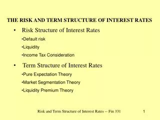
19. Theories of the Term Structure • Three major theories • Expectations • Liquidity Preference • Market Segmentation (Preferred Habitat) • Each of these theories can be used to predict any shaped yield curve.

20. Expectations Theory • Long-term rates are determined by expectations of future short-term rates. • All of the work we have just been doing is based on the expectations hypothesis. • Explaining the yield curve • Upward sloping - future ST rates are expected to increase, thereby increasing LT rates relative to ST • Flat - future ST rates are expected to remain constant • Downward sloping - future ST rates are expected to decrease, thereby decreasing LT rates relative to ST rates

21. Liquidity Preference • This is an extension of the expectations hypothesis. • Long-term rates are based on expected future short-term rates plus a liquidity premium • Investors prefer to invest in the more liquid short-term securities. • To get investors to invest in long-term securities, a higher return, over and above what is expected from the expectations hypothesis, is required

22. Liquidity Preference - Explaining the Yield Curve • upward sloping - Case 1 • Future ST rates are expected to increase • Liquidity premium causes LT rates to be even higher • upward sloping - Case 2 • Future ST rates are expected to decrease • Liquidity premium is large enough to offset decrease in LT rates from expected decline of future ST rates

23. Liquidity Preference - Explaining the Yield Curve • downward sloping • Future ST rates are expected to decrease • Liquidity premium is not large enough to offset decrease in LT rates from expected decline in ST rates • flat • Future ST rates are expected to decrease • Liquidity premium just offsets decrease in LT rates from expected decline in ST rates

24. Preferred Habitat (Market Segmentation) • There are various groups that prefer to invest in a specific maturity range. • The shape of the yield curve will depend on the supply and demand for each maturity range. • Explaining the yield curve • upward sloping - greater demand for ST securities so have to increase LT rates to induce investors to invest in LT securities • downward sloping - greater demand for LT securities so have to increase ST rates to induce investors to invest in ST securities

25. Modern Theories Equilibrium Theories: CIR, BP Non-equilibrium Theories: Dothan, Vasicek, Ho-Lee, Hull-White, HJM Most of them are based on a Brownian Motion as a source of market uncertainty.

26. Brownian Motion B Time

27. Brownian Motion • Starts at the origin • Is continuous • Is normally distributed at each time • Increments are independent • Markovian property • Technical conditions

28. Diffusion Processes General diffusion process: drift noise  - volatility (diffusion parameter)

29. Diffusion Processes  - volatility The major model for stock prices. Why it can NOT be used for bonds?

30. Dothan Model of IR This model gives an analytic pricing formula for bonds, options, but it is not rich enough.

31. Vasicek Model (1977) The Ornstein-Uhlenbeck process with mean reversion.  is the long-run mean. Merton first proposed this process for IR (1971). Extended by Jamshidian for IR options.

32. Cox-Ingersoll-Ross Model The Ornstein-Uhlenbeck process with mean reversion. Merton first proposed this process for IR (1971).

33. HJM=Heat-Jarrow-Morton The most general approach based on a multifactor stochastic model. Very difficult to implement, especially to calibrate. However gives significant advantage in pricing and hedging IR sensitive instruments. Standard implementation via Monte-Carlo.