Download
1 / 153
1.53k likes | 1.85k Vues
Introduction to Risk and return. Chapter 5. Learning Objectives . LO1: The risk-return relationship LO2: Computing the return on a single asset LO3: Evaluating the risk of holding a single asset LO4: Computing the expected return for a portfolio of assets

E N D
Introduction to Risk and return Chapter 5
Learning Objectives • LO1: The risk-return relationship • LO2: Computing the return on a single asset • LO3: Evaluating the risk of holding a single asset • LO4: Computing the expected return for a portfolio of assets • LO5: Evaluating the risk of a portfolio of assets Professor James Kuhle, Ph.D.
The Risk-Return Relationship • Risk • Is determined by the uncertainty of future cash flows • This uncertainty is the result of factors peculiar to each asset Professor James Kuhle, Ph.D.
The Risk-Return Relationship • Investors identify an asset’s risk • Investors subsequently establish a price that compensates them for holding an asset with that level of risk • As risk increases so does the investor’s required return • Investors must be compensated to hold risky assets Professor James Kuhle, Ph.D.
The Risk-Return Relationship • Portfolio risk is harder to measure • Portfolio of assets • A collection of group of assets • Modern portfolio theory • The theory that all investors hold a portfolio of assets called the market portfolio and that risk is measured by the correlation of an asset to this portfolio. • The relationship between risk and return is captured by the CAPM relationship Professor James Kuhle, Ph.D.
L02: Computing the Return on a Single Asset • Computing simple returns • Holding period return (HPR) • consists of earnings from dividends paid, plus the return appreciation or capital gain in the stocks price or Professor James Kuhle, Ph.D.
Computing Simple Returns • The first part of this equation is called capital gain, while the second part is the dividend yield • HPR equals the sum of capital gain and dividend yield Professor James Kuhle, Ph.D.
Average Versus Compound Average • Arithmetic average return • The return calculated where compounding is ignored Professor James Kuhle, Ph.D.
Average Versus Compound Average • Compound (geometric) average return • The return computed that recognizes the interest or earning are paid on accumulated interest or earnings. It is also called geometric return Professor James Kuhle, Ph.D.
Risk and Randomness • Random Variables • Variables with no identifiable relationship between each other • Objects that have more than one possible outcome and for which the magnitude of the outcomes is uncertain beforehand • The possible outcomes are known as states of nature Professor James Kuhle, Ph.D.
Computing Expected Returns • Expected returns reflect the expectations given different possible random outcomes Professor James Kuhle, Ph.D.
LO3: Evaluating Risk of Holding a Single Asset • Standard Deviation • A popular statistical measure that quantifies the dispersion around the expected value • Used to calculate degree of risk • Computing the risk of a single asset • Standard Deviation is a viable method of calculating risk • Greater standard deviation equals greater risk Professor James Kuhle, Ph.D.
Computing the Risk of a Single Asset Professor James Kuhle, Ph.D.
Computing the Standard Deviation Professor James Kuhle, Ph.D.
Computing the Standard Deviation Professor James Kuhle, Ph.D.
Computing the Standard Deviation Professor James Kuhle, Ph.D.
Computing the Standard Deviation Professor James Kuhle, Ph.D.
LO4: Computing the Expected Return for a Portfolio of Assets • A portfolio is a collection of assets • Portfolios can include real estate, stocks, gold, bonds, etc. • The portfolio return is simply a weighted average so the first step is to determine the weights Professor James Kuhle, Ph.D.
Portfolio Weights • How to compute the asset weights for your portfolio • Portfolio weights • The amount invested in asset idivided by the total amount invested in the portfolio Professor James Kuhle, Ph.D.
Computing Portfolio Weights Professor James Kuhle, Ph.D.
Computing Expected Return • Computing expected return with unequal amounts invested in multiple securities Professor James Kuhle, Ph.D.
Computing Expected Return Professor James Kuhle, Ph.D.
LO5: Evaluating the Risk of a Portfolio of Assets • Modern Portfolio Theory shows us that, if we combine assets that are not highly correlated, we can reduce risk. • For example, if one asset is moving up while the other is moving down, these two assets can at least partially offset each other. • Measuring how closely assets are correlated becomes important in constructing a portfolio. Professor James Kuhle, Ph.D.
Evaluating the Risk of a Portfolio of Assets • Correlation • A relationship between observations, in which the movement over time of one item is related to the movement of another • Here’s an example of perfectly negatively correlated returns Professor James Kuhle, Ph.D.
Correlation • Perfectly positively correlated returns Professor James Kuhle, Ph.D.
Diversification Professor James Kuhle, Ph.D.
p Systematic Market = β Assets 5 30 • As we add more stocks to a portfolio the total risk is reduced but cannot be totally eliminated. Unsystematic risk = asset specific
Conclusion about Diversification • Diversification can reduce risk • Risk can never be completely eliminated • Holding multiple risky investments in a portfolio is less risky than each single investment • Assets that are not highly correlated generate the best risk reduction Professor James Kuhle, Ph.D.
Portfolio Theory Chapter 6
Learning Objectives • LO1: Learn about diversification • LO2: Learn about non-diversifiable risk • LO3: Learn about the relationship between non-diversifiable risk and return Prof. James Kuhle, Ph.D.
LO1: Diversification • Diversification • The act of giving something variety • In the context of investing, diversification manages the risk of a portfolio by including a variety of assets • Standard deviation of a two-asset portfolio Prof. James Kuhle, Ph.D.
Portfolio Standard Deviation Prof. James Kuhle, Ph.D.
Portfolio Standard Deviation Prof. James Kuhle, Ph.D.
Portfolio Standard Deviation Prof. James Kuhle, Ph.D.
Types of risk • Non-diversifiable risk • Risk that cannot be eliminated through diversification • Also called systematic risk, and market risk • Measured by beta • Diversifiable risk • Risk that can be eliminated through diversification • Also called unsystematic risk, and firm-specific risk Prof. James Kuhle, Ph.D.
The Market Portfolio • Naïve diversification • The strategy of investing equal amounts of money in a portfolio of randomly selected stocks • Not the most effective approach to portfolio creation • Efficient set • The set of all efficient portfolios across all levels of standard deviation • Harry Markowitz derived a formula for solving for portfolio weights for each of the portfolios in the efficient set • Risk-free asset • An asset with no variation in return and no risk of default • The standard deviation is zero • The correlation of risk-free returns with the returns of any other asset is zero Prof. James Kuhle, Ph.D.
The Market Portfolio • Market portfolio • The value-weighted portfolio that includes every risky asset in the capital markets. • Hypothetical construction of the market portfolio when there are only 2 assets Prof. James Kuhle, Ph.D.
The Market Portfolio • Value-weighted portfolio • In a value-weighted portfolio the portfolio weights are equal to the value of each asset relative to the total value of the assets in the portfolio • Sharpe’s model • Predicts every investor in the capital market has a portfolio with 80% of Big and 20% of Small • Each investor’s portfolio return is equal to the return on the market portfolio Prof. James Kuhle, Ph.D.
The Market Portfolio Proxy • Stock market index • Statistical indicator showing the relative value of a basket of stocks compared to their value in a base year • Measures the ups and downs of the stock market • Serves as a useful proxy for the market portfolio • Exchange traded fund • Seeks to achieve the same return as a particular market index • Unlike indexed mutual funds ETF’s can be traded within a day, shorted, and can be purchased on margin Prof. James Kuhle, Ph.D.
L02: Systematic Risk • Marginal risk • Equal to the covariance between the returns on the asset and the market portfolio • Beta • Measure of systematic risk generated by the capital asset pricing model (CAPM) • Equal to the covariance of returns between the asset and the market portfolio divided by the variance of returns of the market • Measures the amount of systematic risk in a given asset Prof. James Kuhle, Ph.D.
Beta Prof. James Kuhle, Ph.D.
Beta • To estimate beta • Graph the returns on a specific asset (Stock Y) against the returns on the market portfolio (S&P 500 index) • The slope of the line of best fit (ordinary least squares regression line) is beta • The line of best fit, when the return of an asset is plotted against the return on the market portfolio, is also called the characteristic line Prof. James Kuhle, Ph.D.
Beta Prof. James Kuhle, Ph.D.
Estimating Beta Prof. James Kuhle, Ph.D.
Beta Prof. James Kuhle, Ph.D.
Properties of Beta • The market’s beta is equal to 1 • The risk free asset’s beta is equal to 0 • Portfolio beta • The weighted average of the individual betas Prof. James Kuhle, Ph.D.
Portfolio Beta Prof. James Kuhle, Ph.D.
LO3: Equilibrium Risk and Return • Portfolio possibility line • Shows all of the risk and return combinations that can be achieved by forming two-asset portfolios with the risk-free asset and a risky asset • Buying on the margin extends this line • All asset combinations will plot on this line • The slope of this line is called the Treynor Index Prof. James Kuhle, Ph.D.
Treynor Index • Treynor Index • The ratio of the return premium for an asset to its systematic risk (beta) • The return premium is the difference between the expected return on an asset and the return on the risk-free asset • Named after Jack Treynor • Allows you to rank stocks based on return per unit of risk • Let’s look at an example and then add borrowing to the equation Prof. James Kuhle, Ph.D.
Portfolios with the Risk-Free Asset Prof. James Kuhle, Ph.D.