Download
1 / 43
550 likes | 1.29k Vues
MEASURES OF DISPERSION . Handout #7. Measures of Dispersion.

E N D
MEASURES OF DISPERSION Handout #7
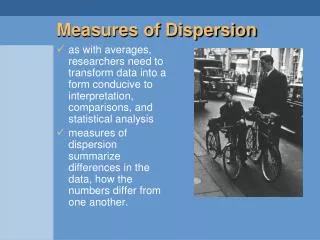
Measures of Dispersion • While measures of central tendency indicate what value of a variable is (in one sense or other) “average” or “central” or “typical” in a set of data, measures of dispersion (or variability or spread) indicate (in one sense or other) the extent to which the observed values are “spread out” around that center — how “far apart” observed values typically are from each other and therefore from some average value (in particular, the mean). Thus: • if all cases have identical observed values (and thereby are also identical to [any] average value), dispersion is zero; • if most cases have observed values that are quite “close together” (and thereby are also quite “close” to the average value), dispersion is low (but greater than zero); and • if many cases have observed values that are quite “far away” from many others (or from the average value), dispersion is high. • A measure of dispersion provides a summary statistic that indicates the magnitude of such dispersion and, like a measure of central tendency, is a univariate statistic.
Importance of the Magnitude Dispersion Around the Average • Dispersion around the mean test score. • Baltimore and Seattle have about the same mean daily temperature (about 65 degrees) but very different dispersions around that mean. • Dispersion (Inequality) around average household income.
Measures of Dispersion • Because dispersion is concerned with how “close together” or “far apart” observed values are (i.e., with the magnitude of the intervals between them), measures of dispersion are defined only for interval (or ratio) variables, • or, in any case, variables we are willing to treat as interval (like IDEOLOGY in the preceding charts). • There is one exception: a very crude measure of dispersion called the variation ratio, which is defined for ordinal and even nominal variables. It will be discussed briefly in the Answers & Discussion to PS #7.) • There are two principal types of measures of dispersion: range measures and deviation measures.
Range Measures of Dispersion • Range measures are based on the distance between pairs of (relatively) “extreme” values observed in the data. • They are conceptually connected with the median as a measure of central tendency. • The (“total” or “simple”) range is the maximum (highest) value observed in the data [the value of the case at the 100th percentile] minus the minimum (lowest) value observed in the data [the value of the case at the 0th percentile] • That is, it is the “distance” or “interval” between the values of the two most extreme cases, • e.g., range of test scores
TABLE 1 – PERCENT OF POPULATION AGED 65 OR HIGHER IN THE 50 STATES (UNIVARIATE DATA) Alabama 12.4 Montana 12.5 Alaska 3.6 Nebraska 13.8 Arizona 12.7 Nevada 10.6 Arkansas 14.6 New Hampshire 11.5 California 10.6 New Jersey 13.0 Colorado 9.2 New Mexico 10.0 Connecticut 13.4 New York 13.0 Delaware 11.6 North Carolina 11.8 Florida 17.8 North Dakota 13.3 Georgia 10.0 Ohio 12.5 Hawaii 10.1 Oklahoma 12.8 Idaho 11.5 Oregon 13.7 Illinois 12.1 Pennsylvania 14.8 Indiana 12.1 Rhode Island 14.7 Iowa 14.8 South Carolina 10.7 Kansas 13.6 South Dakota 14.0 Kentucky 12.3 Tennessee 12.4 Louisiana 10.8 Texas 9.7 Maine 13.4 Utah 8.2 Maryland 10.7 Vermont 11.9 Massachusetts 13.7 Virginia 10.6 Michigan 11.5 Washington 11.8 Minnesota 12.6 West Virginia 13.9 Mississippi 12.1 Wisconsin 13.2 Missouri 13.8 Wyoming 8.9
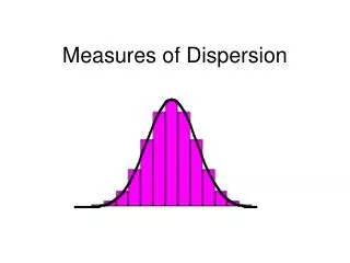
Problems with the [Total] Range • The problem with the [total] range as a measure of dispersion is that it depends on the values of just two cases, which by definition have (possibly extraordinarily) atypical values. • In particular, the range makes no distinction between a polarized distribution in which almost all observed values are close to either the minimum or maximum values and a distribution in which almost all observed values are bunched together but there are a few extreme outliers. • Recall Ideological Dispersion bar graphs => • Also the range is undefined for theoretical distributions that are “open-ended,” like the normal distribution (that we will take up in the next topic) or the upper end of an income distribution type of curve (as in previous slides).
The Interdecile Range • Therefore other variants of the range measure that do not reach entirely out to the extremes of the frequency distribution are often used instead of the total range. • The interdecile range is the value of the case that stands at the 90th percentile of the distribution minus the value of the case that stands at the 10th percentile. • That is, it is the “distance” or “interval” between the values of these two rather less extreme cases.
The Interquartile Range • The interquartile range is the value of the case that stands at the 75th percentile of the distribution minus the value of the case that stands at the 25th percentile. • The first quartile is the median observed value among all cases that lie below the overall median and the third quartile is the median observed value among all cases that lie above the overall median. • In these terms, the interquartile range is third quartile minus the first quartile.
The Standard Margin of Error Is a Range Measure • Suppose the Gallup Poll takes a random sample of n respondents and reports that the President's current approval rating is 62% and that this sample statistic has a margin of error of ±3%. Here is what this means: if (hypothetically) Gallup were to take a great many random samples of the same size n from the same population (e.g., the American VAP on a given day), the different samples would give different statistics (approval ratings), but 95% of these samples would give approval ratings within 3 percentage points of the true population parameter. • Thus, if our data is the list of sample statistics produced by the (hypothetical) “great many” random samples, the margin of error specifies the range between the value of the sample statistic that stands at the 97.5th percentile minus the sample statistic that stands at the 2.5th percentile (so that 95% of the sample statistics lie within this range). Specifically (and letting P be the value of the population parameter) this “95% range” is (P + 3%) - (P -3%) = 6%, i.e., twice the margin error.
Deviation Measures of Dispersion • Deviation measures are based on average deviations from some average value. • Since dispersion measures pertain to with interval variables, we can calculate means, and deviation measures are typically based on the mean deviation from the mean value. • Thus the (mean and) standard deviation measures are conceptually connected with the mean as a measure of central tendency. • Review: Suppose we have a variable X and a set of cases numbered 1,2, . . . , n. Let the observed value of the variable in each case be designated x1, x2, etc. Thus:
Deviation Measures of Dispersion (cont.) • The deviation from the mean for a representative case i is xi - mean of x. • If almost all of these deviations are close to zero, dispersion is small. • If many of these deviations much different from zero, dispersion is large. • This suggests we could construct a measure D of dispersion that would simply be the average (mean) of all the deviations. But this does not work because, as we saw earlier, it is a property of the mean that all deviations from it add up to zero (regardless of how much dispersion there is).
The Mean Deviation • A practical way around this problem is simply to ignore the fact that some deviations are negative while others are positive by averaging the absolute values of the deviations. • This measure (called the mean deviation) tells us the average (mean) amount that the values for all cases deviate (regardless of whether they are higher or lower) from the average (mean) value. • Indeed, the Mean Deviation is an intuitive, understand-able, and perfectly reasonable measure of dispersion, and it is occasionally used in research.
The Variance • Statisticians dislike this measure because the formula is mathematically messy by virtue of being “non-algebraic” (in that it ignores negative signs). • Therefore statisticians, and most researchers, use another slightly different deviation measure of dispersion that is “algebraic.” • This measure makes use of the fact that the square of any real (positive or negative) number other than zero is itself always positive. • This measure --- the average of the squared deviations from the mean (as opposed the average of the absolute deviations) --- is called the variance.
The Variance (cont.) • The variance is the average squared deviation from the mean. • The total (and average) average squared deviation from the mean value of X is smaller than the average squared deviation from any other value of X. • The variance is the usual measure of dispersion in statistical theory, but it has a drawback when researchers want to describe the dispersion in data in a practical way. • Whatever units the original data (and its average values and its mean dispersion) are expressed in, the variance is expressed in the square of those units, which may not make much (or any) intuitive or practical sense. • This can be remedied by finding the (positive) square root of the variance (which takes us back to the original units). • The square root of the variance is called the standarddeviation.
The Standard Deviation (cont.) • In order to interpret a standard deviation, or to make a plausible estimate of the SD of some data, it is useful to think of the mean deviation because • it is easier to estimate (or guess) the magnitude of the MD than the SD; and • the standard deviation has approximately the same numerical magnitude as the mean deviation, though it is almost always somewhat larger. • The SD is never less than the MD; • the SD is equal to the mean deviation if the data is distributed in a maximally “polarized” fashion; • Otherwise the SD is somewhat larger than the MD — typically about 20-50% larger.
Standard Deviation Worksheet • Set up a worksheet like the one shown in the previous slides. • In the first column, list the values of the variable X for each of the n cases. [This is the raw data.] • Find the mean value of the variable in the data, by adding up the values in each case and dividing by the number of cases. • In the second column, subtract the mean from each value to get, for each case, the deviation from the mean. Some deviations are positive, others negative, and (apart from rounding error) they must add up to zero; add them up as an arithmetic check. • In the third column, square each deviation from the mean, i.e., multiply the deviation by itself. Since the product of two negative numbers is positive, every squared deviation is non-negative, i.e., either positive or (in the event a case has a value that coincides with the mean value). • Add up the squared deviations over all cases. • Divide the sum of the squared deviations by the number of cases; this gives the average squared deviation from the mean, commonly called the variance. • The standard deviation is the (positive) square root of the variance. (The square root of x is that number which when multiplied by itself gives x.)
The Mean, Deviations, Variance, and SD • What is the effect of adding a constant amount to (or subtracting from) each observed value? • What is the effect of multiplying each observed value (or dividing it by) a constant amount?
Adding (subtracting) the same amount to (from) every observed value changes the mean by the same amount but does not change the dispersion (for either range or deviation measures)
Multiplying (or dividing) every observed value by the same factor changes the mean and the SD [or MD] by that same factor and changes the variance by that factor squared.
Sample Estimates of Population Dispersion • Random sample statistics that are percentages or averages provide unbiased estimates of the corresponding population parameters. • However, sample statistics that are dispersion measures provide estimates of population dispersion that are biased (at least slightly)downward. • This is most obvious in the case of the range; it should be evident that a sample range is almost always smaller than, and can never be larger than, than the corresponding population range.
Sample Estimates of Population Dispersion (cont.) • The sample standard deviation (or variance) is also biased downward, but only slightly if the sample at all large. • While the SD of a particular sample can be larger than the population SD, sample SDs are on average slightly smaller than the corresponding population SDs). • The sample SD can be adjusted to provide an unbiased estimate of the population SD • This simple adjustment consists of dividing the sum of the squared deviations by n - 1, rather than by n. • Clearly this adjustment makes no practical difference unless the sample is quite small. • Notice that if you apply the SD [or MD or any Range] formula in the event that you have just a single observation in your sample, sample dispersion = 0 regardless of what the observed value is. • More intuitively, you can get no sense of how much dispersion there is in a population with respect to some variable until you observe at least two cases and can see how “far apart” they are. • This is why you will often see the formula for the variance and SD with an n - 1 divisor (and scientific calculators often build in this formula). • However, for POLI 300 problem sets and tests, you should use the formula given in the previous section of this handout.
Dispersion in Ratio Variables • Given a ratio variable (e.g. income), the interesting “dispersion question” may pertain not to the interval between two observed values or between an observed value and the mean value but to the ratio between the two values. • For example, fifty years ago, the income of the household at the 25th percentile was about $5,000 and the income of the household at the 75th percentile was about $10,000, while today the figures are about $40,000 and $80,000 respectively. • While the interval between the two income levels (the interquartile range) has increased from $5,000 to $40,000, the ratio between the two income levels has remained a constant 2 to 1. • Other examples pertain to income: • One household “poverty level” is defined as half of median household income. • Households with more than twice the median income are sometimes characterized as “well off.” • The average compensation of CEOs today is about 250 times that of the average worker, whereas 50 years it was only about 40 times that of the average worker.)
Dispersion in Ratio Variables (cont.) • The degree of dispersion in ratio variables can naturally be referred to as the degree inequality. • For example the two sets of income levels ($5K vs. $10K and $40K vs. $80K) at the 25th and 75th percentiles respectively seem to be “equally unequal” because they are in the same ratio. • Thus the SD does not work well as a measure of inequality (of income, etc.), because it takes no account of the ratio property of [ratio] variables.
The Coefficient of Variation • One ratio measure of dispersion/inequality is called the coefficient of variation, which is simply the standard deviation divided by the mean. • It answers the question: how big is the SD of the distribution relative to the mean of the distribution? • Recall PS#6, Question #7, comparing the distributions of height and weight among American adults. • We naturally to want to say that in some sense that American adults exhibit more dispersion in weight than height. • But if by dispersion we mean [any kind of] range, mean deviation, or variance/SD, the claim is strictly meaningless because the two variables are measured in in different units (pounds, kilograms, etc. vs. inches, feet, centimeters, etc.), so the numerical comparison is not valid.
Coefficient of Variation (cont.) Summary statistics for WEIGHT and HEIGHT (both ratio variables) of American adults in different units: WeightHeight Mean 160 pounds 66 inches 72.6 kilograms 5.5 feet .08 tons 168 centimeters SD 30 pounds 4 inches 13.6 kilograms .33 feet .015 tons 10.2 centimeters Which variable [WEIGHT or HEIGHT] has greater dispersion? [No meaningful answer can be given] Which variable has greater dispersion relative to its average, e.g., greater Coefficient of Dispersion (SD relative to mean)? 30 = 13.6 = .015 = .18 4 = .33 = 10.2 = .06 160 72.6 .08 66 5.5 168 Note that the Coefficient of Variation is a pure number, not expressed in any units and is the same whatever units the variable is measured in.
Coefficient of Variation • The old and new SDs are the same. • The old Coefficient of Variation was SD/Mean = 2/14 = 1/7 = 0.143 • while the new Coefficient of variation is SD/Mean = 2/4 = 0.5
Coefficient of Variation (cont) • The old and new SDs are the same. • The old Coefficient of Variation was • SD/mean = 2/14 = 1/7 = 0.143 • The new Coefficient of Variation is • SD/mean = 2/114 = 0.0175
Coefficient of Variation (cont) • The new SD is 10 times the old SD. • But the old and new Coefficients of Variation are the same: SD/mean = 2/14 = 20/140 = 1/7 = 0.143
The Gini Index • Another measure of dispersion in ratio variables is the Gini Index of Inequality. • The Gini Index is based on a comparison between the actual cumulative distribution when cases are ranked ordered from lowest to highest value (e.g., from poorest to richest) and the cumulative distribution that would exist if all cases had the same value. • Both the Coefficient of Variation and the Gini Index are pure numbers, not expressed in any units ($, pounds, inches, etc.) and unaffected by changing units. • However, the Gini Index is also standardized, with values that range from a minimum of 0 (perfect equality) to a maximum of 1 (perfect inequality).