Chapter 5 CFD Post
Chapter 5 CFD Post. Introduction to CFX. Overview. CFD-Post is a flexible, state-of-the-art post-processor for ANSYS CFD products (CFX and FLUENT) It can run as a standalone post-processor, or within Workbench Includes all the expected plotting objects

Chapter 5 CFD Post
E N D
Presentation Transcript
Chapter 5CFD Post Introduction to CFX
Overview • CFD-Post is a flexible, state-of-the-art post-processor for ANSYS CFD products (CFX and FLUENT) • It can run as a standalone post-processor, or within Workbench • Includes all the expected plotting objects • Planes, Isosurfaces, Vectors, Streamlines, Contours, Animations, … • Allows precise quantitative analysis: • Weighted averages, forces, FFT, results comparison, built-in and user defined macros, … • Can create user defined scalar/vector variables • Includes Automatic Reports, Charts (XY, Time, Histograms), Tables, … • Supports Session files, State files, Command and Expression Languages (including the Perl programming language)
How To Start CFD-Post • Within the CFX-Solver Manager • From the CFX Launcher • Within ANSYS Workbench • From the Start Menu or Command Line • Start > Programs > ANSYS 12.0 > ANSYS CFD-Post
GUI Layout Additional tabs (various tools) Outline tab (“model tree”) Details view Various Viewers (3D, Chart, …)
CFD-Post General Workflow • Prepare locations where data will be extracted from or plots generated • Create variables/expressions which will be used to extract data (if necessary) • i) Generate qualitative data at locations ii) Generate quantitative data at locations • Generate Reports
Creating Locations • Locations are created from the Insert menu or from the toolbar • Once created, all Locations appear as entries in the Outline tree Use the check boxes next to each object in the Outline tree to quickly control visibility Double-click objects in the Outline tree to edit Right-click objects in the Outline tree to Duplicate or Delete
Creating Locations • Domain, Subdomain, Boundary and Mesh Regions are always available • Boundary and Mesh Regions can be edited and coloured by any variable • Mesh Regions provides all available interior/exterior 2D/3D regions from the mesh • All Locations you create are listed under User Locations and Plots • All items contained in the Report are listed here
Location Types • Planes • XY Plane, Point and Normal, etc. • Can define a circle or rectangle to bound the plane, otherwise it’s bounded only by the solution domain(s) • Point • XYZ: At coordinates. Can pick from Viewer • Node Number: Some solver error messages give a node number • Variable Max / Min: Useful to locate where max / min values occur • Point Cloud • Create multiple points • Usually used as seeds to streamlines, vectors
Location Types • Lines • Straight line between two points • Usually used as the basis for an XY Chart • Polylines • Also used for Charts • Read points from a file • Use the line of intersectionbetween a boundary andanother location • Extract a line from acontour plot
Location Types • Volumes • Elements are either in or out • No cut volumes • From Surface • A volume is formed from all elements touching (or above / below) the selected location • Can be useful for mesh checking • Isovolume • Base on a variable at, above or below a given value, or between two values
Location Types Isosurface of pressure behind a flap valve • Isosurfaces • Surface of a variable at a specified value • Iso Clip • An Iso Clip takes a copy of any existing location and then clips it using one or more criteria • E.g. a outlet boundary plot which is then clipped by Velocity >= 10 [m/s] and Velocity <= 20 [m/s] • Can clip using any variable, including geometric variables
Location Types • Vortex Core Region • Used to automatically identify vortex regions • Best method is case dependent • See documentation for details on the different methods • Surface of Revolution • Predefined options for Cylinder, Cone, Disc and Sphere • From Line is much more general • Any line (existing Line, Polyline, Streamline, Particle Track) is rotated about an axis
Location Types • User Surface • Provides a number of additional surface creation options including • From File: reads point data from a text file; usually export this file from a different case • From Contour: extract a contour level • Transformed Surface: rotate, translate or scale an existing surface • Offset From Surface: offset an existing surface in either the Normal direction or by Translating User Surface: From Contour Method (Note: It’s generally easier to use Iso Clips instead)
Colour, Render and View • All Locations have similar Colour, Renderand View settings • Colour • Select the variable with which to colour the location • Set the Range (Global, Local, User Specified) • Pick a Colour Map • Render • Draw Faces: shows solid surface • Draw Lines: shows mesh edges or intersecting lines between mesh edges and the plot • Transparency, Lighting, Texture… • View • Apply Rotation, Translations, Reflection, Scaling • Pick a different Instance Transform
Vector Contour Streamline Particle Track Other Graphics Objects • Insert from the toolbar or the Viewer right-click menus • Vectors, Contour and Streamlines use existing locations as a base • Vector Plot • Can plot any vector variable; usually velocity • Can project vectors Normal or Tangential to the base object • Streamlines • Can proceed forwards and/or backwards from a seeding location • Use the Surface Streamline option to visualise velocity “on” walls
Text Coord Legend Instance Clip Colour Frame Transform Plane Map Other Graphics Objects • Text: add your own labels to the Viewer • Auto-text allows you to show time step/values, expressions, filenames and dates that change automatically • Coord Frame • Legend • Create additional legends that are tied to a specific plot (the default legend changes automatically with the active plot) • Instance Transform • Usually used to re-create full plots from symmetric/periodic solution data
Text Coord Legend Instance Clip Colour Frame Transform Plane Map Other Graphics Objects • Clip Plane • Define a plane; when active all viewer objects in front / behind this plane are hidden • Colour Map • Create custom colour maps
Viewer Right-click Menus • Right-clicking in the Viewer provides a context-sensitive menu • Right-clicking on an object (e.g. Wireframe, Plane) shows options for that object • Can also insert new objects based on the current location • E.g. Insert a vector plot on a Plane • Right-clicking in empty space shows options for the current View • Click on the axes to orientate the view
Variables Tab • The Variables Tab shows information about all available variables • Derived variables • Calculated by CFD-Post – they are not contained in the results file • Geometric variables • X, Y, Z, Normals , mesh quality data • Solution variables • From the results file • User Defined variables • Create new derived variables • Turbo variables • Additional variables automatically created for turbomachinery cases
Variables Tab • The Details pane shows information for the selected variable • Different options for User Defined variables • The Units field allows you to change the units displayed when plotting a variable • You can replace any variable with an expression • New values are stored in the results file, so you can close CFD-Post and the data is retained • Old values can be restored at any time • Example: modifying results for an initial guess • Switch between Hybrid and Conservative variable definitions – see next slide • Only applicable to CFX results • Can also switch between Hybrid and Conservative on the Colour tab for each plot
= Mesh Node = Wall = Mesh Element = Control Volume Boundary = Half Control Volume Adjacent To Wall = Velocity Profile Hybrid vs. Conservative • The finite volumes used by the CFX-Solver are constructed from the mesh, but are not equal to the mesh elements • Mesh nodes lie at the centre of control volumes • Values are stored in the results file at nodes and represent “average” control volume values • Next to wall boundaries you have a half control volume with some representative non-zero velocity • This non-zero velocity is stored at the wall node • But we know that the velocity on a wall is zero • Conservative values = control volume values • Hybrid values = specified boundary condition values
Hybrid Conservative Hybrid vs. Conservative • For visualization purposes, ANSYS CFD-Post uses hybrid values by default, because you usually don’t want to see non-zero wall velocities • For calculation purposes conservative values are used by default • This is good! For example mass flow is calculated correctly — a velocity of zero would produce zero mass flow through the wall adjacent control volume which is clearly wrong • So in most cases you don’t need to worry about Hybrid vs Conservative since CFD-Post does the right thing • User Defined variables will be derived from conservative values by default • Take care when interpreting plots! The range will be different for hybrid and conservative values
Variables Tab: User Defined Variables • Create new variables by Right-click > New… in the top half of the Variables tab • There are 3 methods for User Defined variables • The Expression method defines a variable via an expression, which can be a function of any other variable • Usually create the expression first on the Expressions tab. Example on next slide. • Frozen Copy has been superseded by Case Comparison • The Gradient method calculates the gradient of any existing scalar variable • Produces a new vector variable
User Defined Variables Example • Goal: Plot an isosurface at VelRatio = 0.7 where • On the Expressions tab create the expression for Velocity Ratio: • On the Variables tab create a new variablenamed VelRatio using Method = Expression
User Defined Variables Example • Goal: Plot an isosurface at VelRatio = 0.7 where • Create an Isosurface using the variable VelRatio at a value of 0.7
Expressions Tab • The Expressions tab shows all existing expressions and allows you to create new expressions • Right-click in the top area > New • Enter the new expressions on the Definition tab in the Details view • Right-click to view Functions, Variables etc. that can be used to build your expression • Use the Plot tab to view an XY plot of the expression • Must enter a range for one of the variables and fixed values for the others
Calculators Tab • Function Calculator • Extract engineering data from the results • Many functions, see doc to understand how they operate • Same function used as when creating expressions • Macro Calculator • Run predefined Macros • Write your own Macros and have them appear here • More in Scripting lecture • Mesh Calculator • Mesh quality metrics and stats • Field variables exist for all the metrics and can be plotted
Turbo Post Processing • The Turbo tab contains tools for post-processing turbomachinery cases. See Appendix B for details Specialized turbo charts are generated automatically Blade loading chart
Generating Tables and Charts • Tables and Charts can be created to format and present results
Tables • Select Insert > Table or use the toolbar icon to create a new table • 3D Viewer will switch over to the Table Viewer • Tables allow you to display data and expressions in a tabular view • Tables are automatically added to the Report • Cells can contain expressions or text • Begin with “=“ to distinguish • Expressions are evaluated and updated when variables and/or locations they depend on change • This is not a spreadsheet • Cannot reference other cells 1. Create Table 2. Create Text Cells 3. Create Expression Cells 4. Use drop-down menus to assist expression creation
Charts • Plot a relationship between two variables along a line/curve • Need to create the line first • Polyline, Boundary Intersection curve, Contour line, etc. • Charts are automatically added to the Report • Chart Points are not necessarily evenly spaced • Data points usually correspond to where the line/curve intersects a mesh face • Multiple lines can be plotted on a single chart
Charts 1. Create Curves 2. Create Chart 4. Create Data Series (Lines) 3. Select Chart Type 5. Select X and Y Axis variables
Charts: Type • Charts can be one of three types: • XY • Standard XY plots based on line locators • XY – Transient or Sequence • Plots an expression (usually Time) versus a variable at a point locator • Typically used to show the transient variation of a variable at a point • Data must be present in the trn files • Histogram • Can be based on any locator that contains multiple data locations – lines, surfaces, planes, domains (but not points) • Plots a variable divided into discrete bands on the X Axis versus the frequency of occurrence on the Y Axis
Add new data series Charts: Data Series and Axes • Each data series corresponds to a location (line, point, etc.) which corresponds to a curve on the chart • Use the X and Y Axis tabs to set the variables on the axes • The remaining tabs are for various display options
Fast Fourier Transform • FFT can be applied to signals to extract frequency data Original Signal FFT of Signal Showing Dominant Frequency
Reports • CFD-Post has report generation tools which allow for rapid creation of customized reports • Reports are template based • Depending on the information contained in a results file, a report template will be selected automatically • Right-click on Report to select a different template • You can create your own custom templates or modify existing templates • E.g. add you company logo, add Charts, Tables, Plots etc
Reports • Use the check boxes to control what is included in the report • Double-click items to edit • For example, editing the Mesh Report shows that additional items can be included • Tables and Charts are automatically added to the report. Other items that can be added are Comments and Figures. • Right-click > Insert to add new items • Can also right-click on each item to move it up or down in the report
Reports: Figures • When you add a new Figure it will be listed in the drop-down menu in the top corner of the Viewer • Figures are not static, you can change them after they have been created • If you do not want to change a Figure, make sure one of View 1 – View 4 is selected from the drop down menu • To change the camera position for a figure (i.e. rotate / pan / zoom) select the figure from the Viewer drop down menu and move as necessary • All changes are automatically saved to the Figure
Reports: Figures • When you create a Figure, you have the option to Make copies of objects • If you disable this only the camera and object visibility is stored with the figure • So changing global objects will always cause the Figure to change • Good if you want the Figure to update automatically • If you enable this a local copy of all the current objects is created and shown in the Outline tree • Changing global object will not change the Figure, you must edit the local objects • In both cases the camera position and object visibility can only be changed when the Figure is active
Reports • To view the report, click the Report Viewer tab • After making changes to objects contained in the report you will need to Refresh • Publish writes out an HTML or Text copy of the report • You have the option to generate 3D Viewer files (see below) for all Figures
Other Tools • Timestep Selector • Transient results are post-processed by loading in the end results file, then selecting different timesteps from the Timestep Selector • Animation • Animate objects, create MPEGs • More on next slide • Quick Editor • Provides a very quick way to change the “primary” value associated with each object • Probe • Pick a point from the Viewer and probe a variable value at that point Timestep Animation Quick Probe Selector Editor
Animations • Animations have two modes, Quick and Keyframe • In Quick Animation mode you simply pick an object and click the Play button • The “primary” variable for that object is animated • Limited control • Keyframe mode gives you much more control • When you create a Keyframe a snapshot of the current state is stored with that Keyframe • A series of Keyframes represent a series of different states • Camera position, object visibility, selected timestep, or anything else can be different between Keyframes • An animation needs at least two Keyframes (one for the start and one for the end) • Enter the # of Frames between each Keyframe • Everything that is different between the Keyframes gets interpolated over the # of Frames
Typical Keyframe Animation Procedure • Using the Timestep Selector load the first timestep • Create necessary plots and position the view • Create the first Keyframe • Load the last timestep • If necessary change the plots and the view • Create the second Keyframe • Select the first Keyframe and set the # of Frames • This is the # of Frames in between the first and second Keyframes • If we have a total of 100 timesteps, then setting # of Frames to 98 will produce a total of 100 frames (98 plus first, plus last) and therefore 1 frame per timestep • Set the Movie options • Rewind to the first Keyframe and click Play In this example the first and second Keyframes used a different view position and the Transparency of the Plane was changed from 0 to 1. The changes between Keyframes are interpolated gradually over each animation frame
Multi File Mode • To post-process multiple files simultaneously you can: • Multi-select files when loading • Load a multi-configuration results file (.mres) using Load complete history as> Separate Cases • Or load additional results and enable the Keep current cases loaded toggle • Each file is shown separately in the Outline tree and the Viewer • Sync cameras • All Views move the same • Sync objects • The visibility of all User Locations and Plots is the same
SST k-e Difference Plot Case Comparison • When multiple files are loaded you can select Case Comparison from the Outline tree • Automatically generates difference variables and plots • Expression syntax: • function()@CASE:#.Location • E.g: areaAve(Pressure)@CASE:1.Inlet
3D Viewer Files • Save Picture in the CFX Viewer State (3D) file format (.cvf file) • Can then use the stand-alone Viewer to view the file, rotate, pan, zoom, etc • Unlicensed and free to distribute to your customers • Can embed 3D Viewer files in PowerPoints and HTML files • Download from the Customer Portal under Product Information > ANSYS CFX Zoom
FLUENT Results • All CFD-Post features are available for FLUENT case and data files • All mesh types supported • Polyhedral, non-conformal, adapted, ... • 2D FLUENT meshes are extruded to thin 3D domains • 2D axisymmetric meshes are converted to 3D wedges • Limitations: • Some data may not be in the standard .dat file • Export through the Data File Quantities or the Export to CFD-Post panels • Data that is not field data, such as particle locations and tracks, cannot be visualized in CFD-Post at present • Model set-up information is not available in CFD-Post • CFD-Post is serial, not parallel Polyhedral mesh case 2D to Thin 3D
Files • CFD-Post can interact with a number of different files including: • Results Files • CFX .res / .mres, ANSYS .rst, FLUENT.dat • Mesh Files • CFX .def / .mdef, ANSYS .cmdb, FLUENT .cas, • Import • Polyline .csv, User Surface .csv, ANSYS surface .cdb • Export • Profile Data .csv, General Formatted Results .csv,ANSYS load file .csv • Recorded Session Files (.cse) • State Files (.cst) • Macros (.cse)
Files • Results • ANSYS • CFD-Post is able to read ANSYS results for temperature, velocity, acceleration, magnetic forces, stress, strain, and mesh deformation • Import • Locations: .csv files which contain point data which defines a polyline or surface • ANSYS Surface Mesh (.cdb): To allow for export of data on a surface for use as a boundary condition in ANSYS • Export • Profile Boundary Data: for use in CFX-Pre • General formatted results data • ANSYS Load Data: Written onto an imported ANSYS .cdb file
Files • Session • Session files can be used to quickly reproduce all the actions performed in a previous CFD-Post session • Session recording in CFX Command Language (CCL) • State • Saves a snap-shot of all objects • Use to re-load all post-processing objects that existed when the state file was saved • Are not tied to a particular file • But work best when region names are consistent • Excludes actions (e.g. file output) • Macro • More later in Scripting and Automation lecture