Nanoscale Digital Computation Through Percolation
230 likes | 255 Vues
Nanoscale Digital Computation Through Percolation. Mustafa Altun Electrical and Computer Engineering. University of Minnesota. DAC, “Wild and Crazy Ideas” Session ─ San Francisco, July 29, 2009. Non-Linearities.

Nanoscale Digital Computation Through Percolation
E N D
Presentation Transcript
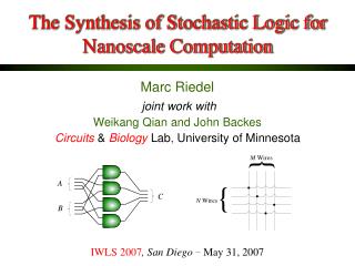
Nanoscale Digital Computation Through Percolation Mustafa Altun Electrical and Computer Engineering Universityof Minnesota DAC, “Wild and Crazy Ideas” Session ─ San Francisco, July 29, 2009
Non-Linearities From vacuum tubes, to transistors, to carbon nanotubes, the basis of digital computation is a robust non-linearity. signal out Holy Grail signal in
Randomness at the Nanoscale General Characteristics of Nanoscale Circuits: • Self-assembled topologies. • High densityof bits/ logic/interconnects. • High defect and failure rates. • Inherent randomness in both interconnects and signal values. Probabilistic FET-like connections in a stochastically assembled nanowire array.
Nanoscale Computation through Percolation • Given: Physical structures exhibiting randomness. • Want: Robust digital computation. • “WACI” idea: Exploit the mathematics of percolation.
Percolation Theory Rich mathematical topic that forms the basis of explanations of physical phenomena such as diffusion and phase changes in materials. Sharp non-linearity in global connectivity as a function of random local connectivity. RandomGraphs Broadbent & Hammersley (1957); Kesten (1982); and Grimmett (1999).
D S Percolation Theory Poisson distribution of points with density λ Points areconnectedif their distance is less than2r Study probabilityof connected components
Percolation Theory There is a phase transition at a critical node density value.
Nanowire crossbar arrays signal in signal out • Suppose that, in this technology, crosspoints are FET-like junctions. • When a high or low voltage is applied, these develop low or high impedances, respectively. 8
Crosspoints as squares We model each crosspoint as a square. (Black corresponds to ON; white corresponds to OFF.) 9
Implementing Boolean functions signals in: Xij’s signals out: connectivity top-to-bottom / left-to-right. 10
An example with 16 Boolean inputs A path exists between top and bottom, f = 1 11
An example on 2×2 array Relation between p1─ probability of experiencing ON crosspoint ─ and switch’s behavior. • If p1 is 0.9 then the switch is ON with probability 95%. (The probability of getting an error is 5%.) • If p1 is 0.1, the switch is OFF with probability 95%. (The probability of getting an error is 5%.) 12
Non-Linearity Through Percolation p2 p1 p2versusp1for 1×1, 2×2, 6×6, 24×24, 120×120, and infinite size lattices. • Each square in the lattice is colored black with independent probability p1. • p2 is the probability that a connected path exists between the top and bottom plates. 13
Defects matter! • Ideally, if the applied voltage is 0, then all the crosspoints are OFF and so there is no connection between any of the plates. • Ideally, If the applied voltage is VDD, then all the crosspoints are ON and so the plates are connected. • With defect in nanowires, not all crosspoints will respond this way. 14
Margins • One-margin: Tolerable p1 ranges for which we interpret p2 as logical one. • Zero-margin: Tolerable p1 ranges for which we interpret p2 as logical zero. Margins correlate with the degree of defect tolerance. 15
Margin performance with a 2×2 lattice f =X11X21+X12X22 g =X11X12+X21X22 Different assignments of input variables to the regions of the network affect the margins. 16
One-margins (always good) ONE-MARGIN f =1 f =0 Defect probabilities exceeding the one-margin would likely cause an (1→0) error. 17
Good zero-margins ZERO-MARGIN f =0 f =1 Defect probabilities exceeding zero-margin would likely cause an (0→1) error. 18
Poor zero-margins POOR ZERO-MARGIN f =1 f =0 Assignments that evaluate to 0 but have diagonally adjacent assignments of blocks of 1's result in poor zero-margins 19
Lattice duality • Note that each side-to-side connected path corresponds to the AND of the inputs; the paths taken together correspond to the OR of these AND terms, so implement a sum-of-products expression. • A necessary and sufficient condition for good error margins is that the Boolean functions corresponding to the top-to-bottom and left-to-right plate connectivities f and g are dual functions.
Further work • Solve the logic synthesis problem. (Bring continuum mathematics into the field.) • Explore physical implementation in nanowire arrays. • Explore percolation as a model for digital computation with DNA and other molecular substrates.
Funding MARCO (SRC/DoD) Contract #NT-1107 NSF CAREER Award #0845650