Integrated Learning Center: Introduction to Statistics for Social Sciences
Welcome to the Spring 2014 course "Introduction to Statistics for the Social Sciences" at the Integrated Learning Center (ILC). This course, conducted in Room 120, features lectures three times a week aimed at equipping students with the statistical skills necessary for analyzing social science data. Key topics include hypothesis testing, correlations, and regression analysis. Labs continue this week, and prior readings are essential for success. Stay on top of your assignments to fully grasp the statistical tools we will utilize throughout the semester.

Integrated Learning Center: Introduction to Statistics for Social Sciences
E N D
Presentation Transcript
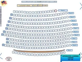
Screen Cabinet Cabinet Lecturer’s desk Table Computer Storage Cabinet Row A 3 4 5 19 6 18 7 17 16 8 15 9 10 11 14 13 12 Row B 1 2 3 4 23 5 6 22 21 7 20 8 9 10 19 11 18 16 15 13 12 17 14 Row C 1 2 3 24 4 23 5 6 22 21 7 20 8 9 10 19 11 18 16 15 13 12 17 14 Row D 1 2 25 3 24 4 23 5 6 22 21 7 20 8 9 10 19 11 18 16 15 13 12 17 14 Row E 1 26 2 25 3 24 4 23 5 6 22 21 7 20 8 9 10 19 11 18 16 15 13 12 17 14 Row F 27 1 26 2 25 3 24 4 23 5 6 22 21 7 20 8 9 10 19 11 18 16 15 13 12 17 14 28 Row G 27 1 26 2 25 3 24 4 23 5 6 22 21 7 20 8 9 29 10 19 11 18 16 15 13 12 17 14 28 Row H 27 1 26 2 25 3 24 4 23 5 6 22 21 7 20 8 9 10 19 11 18 16 15 13 12 17 14 Row I 1 26 2 25 3 24 4 23 5 6 22 21 7 20 8 9 10 19 11 18 16 15 13 12 17 14 1 Row J 26 2 25 3 24 4 23 5 6 22 21 7 20 8 9 10 19 11 18 16 15 13 12 17 14 28 27 1 Row K 26 2 25 3 24 4 23 5 6 22 21 7 20 8 9 10 19 11 18 16 15 13 12 17 14 Row L 20 1 19 2 18 3 17 4 16 5 15 6 7 14 13 INTEGRATED LEARNING CENTER ILC 120 9 8 10 12 11 broken desk
Introduction to Statistics for the Social SciencesSBS200, COMM200, GEOG200, PA200, POL200, or SOC200Lecture Section 001, Spring, 2014Room 120 Integrated Learning Center (ILC)10:00 - 10:50 Mondays, Wednesdays & Fridays. Welcome http://www.youtube.com/watch?v=oSQJP40PcGI
Please click in My last name starts with a letter somewhere between A. A – D B. E – L C. M – R D. S – Z
Lab sessions Labs continue this week
Schedule of readings Before next exam (Monday May 5th) Please read chapters 10 – 14 Please read Chapters 17, and 18 in Plous Chapter 17: Social Influences Chapter 18: Group Judgments and Decisions
For our class Due Monday April 28th
For our class Due Monday April 28th
Homework due – Wednesday (April 23rd) • On class website: • Please print and complete homework worksheet #21 • Regression
Use this as your study guide Next couple of lectures 4/21/14 Logic of hypothesis testing with Correlations Interpreting the Correlations and scatterplots Simple and Multiple Regression Using correlation for predictions r versus r2 Regression uses the predictor variable (independent) to make predictions about the predicted variable (dependent)Coefficient of correlation is name for “r”Coefficient of determination is name for “r2”(remember it is always positive – no direction info)Standard error of the estimate is our measure of the variability of the dots around the regression line(average deviation of each data point from the regression line – like standard deviation) Coefficient of regression will “b” for each variable (like slope)
Regression Example Rory is an owner of a small software company and employs 10 sales staff. Rory send his staff all over the world consulting, selling and setting up his system. He wants to evaluate his staff in terms of who are the most (and least)productive sales people and also whether more sales calls actually result in more systems being sold. So, he simply measures the number of sales calls made by each sales person and how many systems they successfully sold. Review
50 40 Number of systems sold 30 20 10 0 0 1 2 3 4 Number of sales calls made Ava 70 Emily Regression Example Isabella 60 Do more sales calls result in more sales made? Emma Step 1: Draw scatterplot Ethan Step 2: Estimate r Joshua Jacob Dependent Variable Independent Variable Review
Regression: Predicting sales Step 1: Draw prediction line r = 0.71 b= 11.579 (slope) a = 20.526 (intercept) Draw a regression line and regression equation What are we predicting? Review
Assumptions Underlying Linear Regression • For each value of X, there is a group of Y values • These Y values are normally distributed. • The means of these normal distributions of Y values all lie on the straight line of regression. • The standard deviations of these normal distributions are equal.
Residuals: Evaluating Staff Step 1: Compare expected sales levels to actual sales levels 70-55.3=14.7 Difference between expected Y’ and actual Y is called “residual” (it’s a deviation score) Ava 14.7 How did Ava do? Ava sold 14.7 more than expected taking into account how many sales calls she made over performing Review
Residuals: Evaluating Staff Step 1: Compare expected sales levels to actual sales levels 20-43.7=-23.7 Difference between expected Y’ and actual Y is called “residual” (it’s a deviation score) Ava How did Jacob do? -23.7 Jacob sold 23.684 fewer than expected taking into account how many sales calls he made under performing Jacob Review
Residuals: Evaluating Staff Step 1: Compare expected sales levels to actual sales levels Difference between expected Y’ and actual Y is called “residual” (it’s a deviation score) Ava 14.7 Emma Isabella Emily Madison -23.7 Joshua Jacob Review
Residuals: Evaluating Staff Step 1: Compare expected sales levels to actual sales levels Difference between expected Y’ and actual Y is called “residual” (it’s a deviation score) Ava 14.7 Emma Isabella -6.8 Emily Madison -23.7 7.9 Joshua Jacob Review
Does the prediction line perfectly the predicted variable when using the predictor variable? No, we are wrong sometimes… How can we estimate how much “error” we have? Difference between expected Y’ and actual Y is called “residual” (it’s a deviation score) 14.7 The green lines show how much “error” there is in our prediction line…how much we are wrong in our predictions -23.7 Perfect correlation = +1.00 or -1.00 Each variable perfectly predicts the other No variability in the scatterplot The dots approximate a straight line
How do we find the average amount of error in our prediction Deviation scores Diallo is 0” Preston is 2” Mike is -4” Step 1: Find error for each value (just the residuals) Hunter is -2 Y – Y’ Sound familiar?? Step 2: Find average √ Difference between expected Y’ and actual Y is called “residual” (it’s a deviation score) ∑(Y – Y’)2 n - 2 How would we find our “average residual”? Σx The green lines show how much “error” there is in our prediction line…how much we are wrong in our predictions N
Standard error of the estimate (line) = These would be helpful to know by heart – please memorize these formula
Regression Analysis – Least Squares Principle When we calculate the regression line we try to: • minimize distance between predicted Ys and actual (data) Y points (length of green lines) • remember because of the negative and positive values cancelling each other out we have to square those distance (deviations) • so we are trying to minimize the “sum of squares of the vertical distances between the actual Y values and the predicted Y values”
Which minimizes error better? Is the regression line better than just guessing the mean of the Y variable?How much does the information about the relationship actually help? How much better does the regression line predict the observed results? r2 Wow!
What is r2? r2 = The proportion of the total variance in one variable that is predictable by its relationship with the other variable Examples If mother’s and daughter’s heights are correlated with an r = .8, then what amount (proportion or percentage) of variance of mother’s height is accounted for by daughter’s height? .64 because (.8)2 = .64
What is r2? r2 = The proportion of the total variance in one variable that is predictable for its relationship with the other variable Examples If mother’s and daughter’s heights are correlated with an r = .8, then what proportion of variance of mother’s height is not accounted for by daughter’s height? .36 because (1.0 - .64) = .36 or 36% because 100% - 64% = 36%
What is r2? r2 = The proportion of the total variance in one variable that is predictable for its relationship with the other variable Examples If ice cream sales and temperature are correlated with an r = .5, then what amount (proportion or percentage) of variance of ice cream sales is accounted for by temperature? .25 because (.5)2 = .25
What is r2? r2 = The proportion of the total variance in one variable that is predictable for its relationship with the other variable Examples If ice cream sales and temperature are correlated with an r = .5, then what amount (proportion or percentage) of variance of ice cream sales is not accounted for by temperature? .75 because (1.0 - .25) = .75 or 75% because 100% - 25% = 75%
Some useful terms • Regression uses the predictor variable (independent) to make predictions about the predicted variable (dependent) • Coefficient of correlation is name for “r” • Coefficient of determination is name for “r2”(remember it is always positive – no direction info) • Standard error of the estimate is our measure of the variability of the dots around the regression line(average deviation of each data point from the regression line – like standard deviation)
+0.92 positive strong The relationship between the hours worked and weekly pay is a strong positive correlation. This correlation is significant, r(3) = 0.92; p < 0.05 up down 55.286 6.0857 y' = 6.0857x + 55.286 207.43 85.71 .846231 or 84% 84% of the total variance of “weekly pay” is accounted for by “hours worked” For each additional hour worked, weekly pay will increase by $6.09
400 380 360 Wait Time 340 320 300 280 7 8 6 5 4 Number of Operators
Critical r = 0.878 No we do not reject the null -.73 negative strong The relationship between wait time and number of operators working is negative and moderate. This correlation is not significant, r(3) = 0.73; n.s. number of operators increase, wait time decreases 458 -18.5 y' = -18.5x + 458 365 seconds 328 seconds .53695 or 54% The proportion of total variance of wait time accounted for by number of operators is 54%. For each additional operator added, wait time will decrease by 18.5 seconds
39 36 33 30 27 24 21 Percent of BAs 45 48 51 54 57 60 63 66 Median Income
Critical r = 0.632 Yes we reject the null Percent of residents with a BA degree 10 8 0.8875 positive strong The relationship between median income and percent of residents with BA degree is strong and positive. This correlation is significant, r(8) = 0.89; p < 0.05. median income goes up so does percent of residents who have a BA degree 3.1819 0.0005 y' = 0.0005x + 3.1819 25% of residents 35% of residents .78766 or 78% The proportion of total variance of % of BAs accounted for by median income is 78%. For each additional $1 in income, percent of BAs increases by .0005
30 27 24 21 18 15 12 Crime Rate 45 48 51 54 57 60 63 66 Median Income
Critical r = 0.632 No we do not reject the null Crime Rate 10 8 -0.6293 negative moderate The relationship between crime rate and median income is negative and moderate. This correlation is not significant, r(8) = -0.63; p < n.s. [0.6293 is not bigger than critical of 0.632] . median income goes up, crime rate tends to go down 4662.5 -0.0499 y' = -0.0499x + 4662.5 2,417 thefts 1,418.5 thefts .396 or 40% The proportion of total variance of thefts accounted for by median income is 40%. For each additional $1 in income, thefts go down by .0499
Thank you! See you next time!!