Download
1 / 27
280 likes | 418 Vues
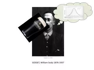
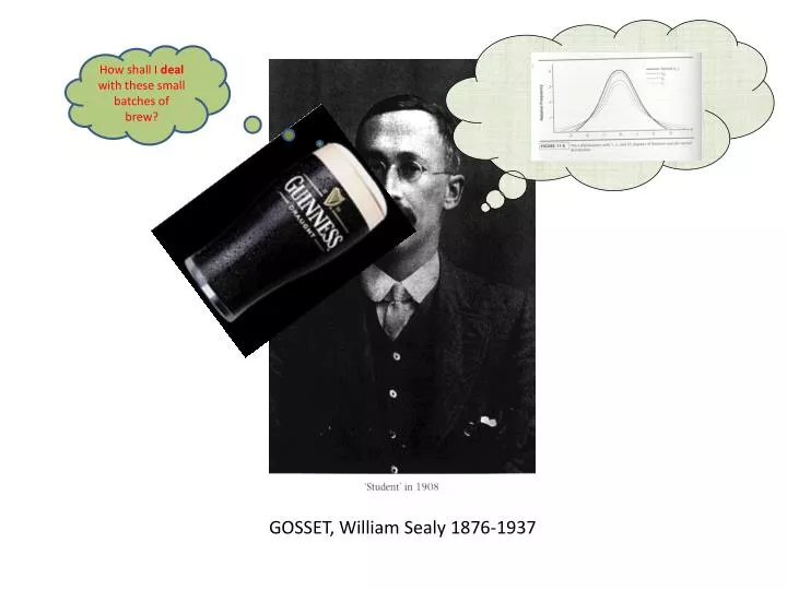
How shall I deal with these small batches of brew?. GOSSET, William Sealy 1876-1937.

E N D
How shall I deal with these small batches of brew? GOSSET, William Sealy 1876-1937
A series of distributions of sample means drawn from a population of standardized scores (therefore the mean of mean is 0 and sd=1), in which the shape of the distribution varies systematically, depending on the size of the sample. The larger the sample, the more it matches a normal distribution; and the smaller the sample, the fatter the tails. GOSSET, William Sealy 1876-1937
A T distribution is derived by approximating the mean of a normally distributed population, particularly useful with an unknown standard deviation and a small sample size. To visualize how it functions, imagine an inverted letter T placed under this standard probability distribution, where the Two Tails of this inverted T are nestled within the Two Tails of the standard probability distribution, thus making the Two Tails Thicker than a Typical distribution. As the sample size rises, the range of potential outlier sample means derived from the population shortens; therefore, the Two Tails of the probability distribution shorten (along with the standard deviation) and Thus Thrust into the Two Tails of the inverted T, also causing the inverted T to rise and create a greater kurTosis Jeremy Jimenez
XY XY XY XY XY XY XY XY XY XY XY XY XY XY XY XY XY XY XY XY XY XY XY XY XY XY XY XY XY XY XY XY XY XY XY XY XY XY XY XY XY XY ρ
SampleC SampleD rXY Population rXY SampleB XY rXY SampleE SampleA _ rXY rXY
r N - 2 t = 1 - r2 The t distribution, at N-2 degrees of freedom, can be used to test the probability that the statistic r was drawn from a population with = 0. Table C. H0 : XY = 0 H1 : XY 0 where
Monday, November 7 Independent samples t-test for the difference between two means.
Monday, November 7 Independent samples t-test for the difference between two means. signal-to-noise ratio
Monday, November 7 Independent samples t-test for the difference between two means. signal-to-noise ratio safety in numbers
_ _ _ _ _ _ _ _ _ _ _ _ _ _ _ _ _ _ _ _ _ _ _ _ X1- X2 X1- X2 X1- X2 X1- X2 X1- X2 X1- X2 X1- X2 X1- X2 X1- X2 X1- X2 X1- X2 X1- X2 X1-X2 μ1- μ2
H0 : 1 - 2 = 0 H1 : 1 - 2 0
_ _ Xgirls=51.16 Xboys=53.75 How do we know if the difference between these means, of 53.75 - 51.16 = 2.59, is reliably different from zero?
_ _ Xgirls=51.16 Xboys=53.75 We could find confidence intervals around each mean... 95CI: 52.07 boys 55.43 95CI: 49.64 girls 52.68
H0 : 1 - 2 = 0 H1 : 1 - 2 0 But we can directly test this hypothesis...
H0 : 1 - 2 = 0 H1 : 1 - 2 0 To test this hypothesis, you need to know … …the sampling distribution of the difference between means. - - X1-X2
H0 : 1 - 2 = 0 H1 : 1 - 2 0 To test this hypothesis, you need to know … …the sampling distribution of the difference between means. - - X1-X2 …which can be used as the error term in the test statistic.
The sampling distribution of the difference between means. X1-X2 = 2X1 +2X2 - - - - This reflects the fact that two independent variances contribute to the variance in the difference between the means.
The sampling distribution of the difference between means. X1-X2 = 2X1 +2X2 - - - - This reflects the fact that two independent variances contribute to the variance in the difference between the means. Your intuition should tell you that the variance in the differences between two means is larger than the variance in either of the means separately.
(X1 - X2) z = X1-X2 The sampling distribution of the difference between means, at n = , would be: - - - -
The sampling distribution of the difference between means. - - X1-X2 = 21 22 + n1n2 Since we don’t know , we must estimate it with the sample statistic s.
The sampling distribution of the difference between means. - - X1-X2 = s21 s22 + n1n2 Rather than using s21 to estimate 21 and s22 to estimate 22 , we pool the two sample estimates to create a more stable estimate of 21 and 22 by assuming that the variances in the two samples are equal, that is, 21 = 22 .
sp2 sp2 sX1-X2 = + N 1 N2
sp2 sp2 sX1-X2 = + N1 N2
SSw SS1 + SS2 sp2 = = N-2N-2 sp2 sp2 sX1-X2 = + N1 N2
(X1 - X2) - (1 - 2 ) t = sX1-X2 Because we are making estimates that vary by degrees of freedom, we use the t-distribution to test the hypothesis. …at (n1 - 1) + (n2 - 1) degrees of freedom (or N-2)
Assumptions • X1 and X2 are normally distributed. • Homogeneity of variance. • Samples are randomly drawn from their respective populations. • Samples are independent.