… cannot be analyzed on common time windows ,

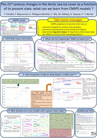
1. The 21stcentury changes in the Arcticseaicecover as a function of itspresent state: whatcanwelearnfrom CMIP5 models ? T. Fichefet, F. Massonnet, G. Philippon-Berthier, C. Bitz, M. Holland, H. Goosse, P. -Y. Barriat Take home messages CMIP5 setup … cannotbeanalyzed on common time windows, … cannotbeconstrained by current trends (not robust), … have similarlong-termslopes importance of the mean state, … are shifted in time but show resembling patterns. CMIP5 projections of summerArcticseaice Multi-model mean NSIDC (Fetterer et al., 2002) • 18 Earth System and General Circulation Models. • 2 Representative Concentration Pathways (RCP4.5/8.5, Moss et al., 2010). • Arcticseaiceonly, work on each model grid. • « SSIE »=Septemberseaiceextent. 1. 1979-2010 mean and trends 2. Whatwill the September 2060 iceextentbe? Arctic Sept. iceextent - RCP4.5 Arctic Sept. iceextent - RCP8.5 mean of members mean of members member member Multi-model mean Obs. ± 2σuncertaintyinterval • In 2060 (an example date), somemodels are alreadyatnearice-free conditions, other are stilllosingice. It does not makesense to compare modelsatthat time and, evenworse, to look at the multi-model mean! • For thesereasons, there are no systematic and clearrelationshipsbetween initial state (extent, thickness,…) and future changes of Septemberextent, because the models are not synchronized. • Instead of lookingatchanges over a certain time period, we propose to look at the time taken to reach a certain thresholdextent. • Reasonablesimulatedmeanextent in summer. • Underestimation of the trend over 1979-2010 (OK over 1979-2006, improvementw.r.t. CMIP3 on thatperiod (Stroeve et al., 2007)). • Membersclustered for the mean, scattered for the trends. 3. How long doesittake to drop below 1 million km² ? • Fig. 4: Corrrelations(y-axis) , across the CMIP5 models, between • the year of lowiceextent(YLE), i.e. the yearatwhich SSIE drops below a givenextent (θ, x-axis), and • the initial mean state over 1979-2010: SSIE (thick+bulletlines), annualmeanicethickness (thickdashed), Septemberthinice (<0.5m) extent (thin), and amplitude of the seasonal cycle of iceextent (thindashed). • The procedureisrepeated for RCP4.5and RCP8.5. The time taken to reach a givenextentis a linearfunction of the initial summerextent. Yetapparently trivial, thisapproach has the advantage to compare modelswhenthey have similarmean states, and not at a given time. Inter-model (x) correlation: 0.82 RCP8.5 • The relationships are valid for the twoRCPs, otherinitial variables, and otherthresholds. Septemberseaiceextentisdroppingbelow a giventhresholdearlier in the 21st centurywhen: • the initial SSIE islower, • the initial seaicecoveristhinner on average, • the extentcovered by thinice (<0.5m) islarger, • the amplitude of the seasonal cycle of seaiceextentislarger. YearatwhichSeptemberextent < 1 million km² 1979-2010 meanSeptemberseaiceextent (106 km²) 4. Whyshould one trust modelswith a good mean state? Additional info 1 Because the CMIP5 models have a similarlong-termtrend of SSIE (see frames 2 and 3), but scatteredshort-termtrends (frame 1), itislikelythat trends of SSIE in each model must atsome point adjust to the common long-term trend. This isachieved by a rapidloss of ice, at a timing peculiar to each model (indicated by the vertical dashedlines, Figure on the left), but at a common, critical SSIE (≈ 3 million km²). Giventhat the time to reachthiscriticalextentis a function of the initial mean state (frame 3), werecommendevaluatingmodels on theirmean state. According to the 6 modelsselected on the left, SSIE permanently drops below 1 million km² between 2049 (earlier model) and 2077 (later model), under RCP8.5. Note: for RCP4.5, similar conclusions hold for modelswith few icenow (the othersdon’treach 3 million km² before 2100). References -F. Fetterer, K. Knowles, W. Meier, M. Savoie, Seaice index(electronicreference) (2002) http://nsidc.org/data/docs/noaa/g02135_seaice_index/ -R. J. Moss et al., The nextgeneration of scenarios for climate change research and assessment, Nature, 2010. -J. Stroeve, M. M. Holland, W. meier, T. Scambos, M. Serreze,Arcticseaicedecline: fasterthanforecast, GRL, 2007 -J. E. Kay, M. M. Holland, A. Jahn, Interannual to multidecadalArcticseaiceextent trends in a warming world, GRL, 2011. Affiliations TF, FM, GPB, HG, PYB: Georges Lemaître Centre for Earth and ClimateResearch, Earth and Life Institute, Université catholique de Louvain, Belgium CB: Department of Atmospheric Sciences, University of Washington, Washington MH: National Center for AtmosphericResearch, Colorado Contacts francois.massonnet@uclouvain.be www.climate.be/u/fmasson thierry.fichefet@uclouvain.be 0 Running trends of othermodels Running trends of modelswith SSIE or amplitude of seasonal cycle extentin the range of observations -1 EC-Earth -2 1 0 1 -1 0 bcc-csm1-1 GISS-E2-R CanESM2 -2 -1 1 HadGEM2-CC IPSL-CM5A-MR Trend over the previous 32 years (106 km²/10y) -2 0 1 -1 inmcm4 CSIRO-Mk6-3-0 CNRM-CM5 0 -2 Trend over the previous 32 years (106 km²/10y) -1 1 CCSM4 MPI-ESM-LR -2 0 On the contrary, the 1979-2010 trends should not beusedto constrain projections: for current, observedmean SSIE, these are too volatile statistics (see the members of the samemodels, frame 1), consistently with Kay et al., 2011. If the observed trends happen to beat the tail of the distribution due to the highnaturalvariability, thenwewillreject good models for wrongreasons. -1 Figure: Running trends of CMIP5 models SSIE underhistorical + RCP8.5 forcings. HadGEM2-ES MRI-CGCM3 NorESM1-M -2 1 0 -1 MIROC5 GFDL-ESM2M IPSL-CM5A-LR -2 1900 2100 1900 2000 2100 1900 2000 2100 2000