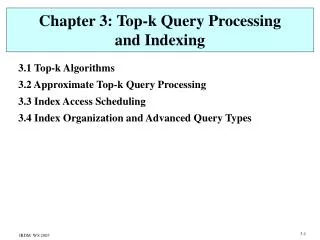
Chapter 3: Top-k Query Processing and Indexing
Chapter 3: Top-k Query Processing and Indexing. 3.1 Top-k Algorithms 3.2 Approximate Top-k Query Processing 3.3 Index Access Scheduling 3.4 Index Organization and Advanced Query Types. 3.1 Top-k Query Processing with Scoring. Vector space model suggests m ×n term-document matrix ,

Chapter 3: Top-k Query Processing and Indexing
E N D
Presentation Transcript
Chapter 3: Top-k Query Processing and Indexing 3.1 Top-k Algorithms 3.2 Approximate Top-k Query Processing 3.3 Index Access Scheduling 3.4 Index Organization and Advanced Query Types
3.1 Top-k Query Processing with Scoring Vector space model suggests m×n term-document matrix, but data is sparese and queries are even very sparse better use inverted index lists with terms as keys for B+ tree q: professor research xml B+ tree on terms ... ... professor research xml 17: 0.3 17: 0.3 12: 0.5 11: 0.6 index lists with (DocId, s = tf*idf) sorted by DocId 44: 0.4 44: 0.4 14: 0.4 17: 0.1 17: 0.1 Google: > 10 mio. terms > 8 bio. docs > 4 TB index 52: 0.1 28: 0.1 28: 0.7 ... 53: 0.8 44: 0.2 44: 0.2 55: 0.6 51: 0.6 ... 52: 0.3 ... terms can be full words, word stems, word pairs, word substrings, etc. (whatever „dictionary terms“ we prefer for the application) queries can be conjunctive or „andish“ (soft conjunction)
q: professor research xml DBS-Style Top-k Query Processing B+ tree on terms ... ... professor research xml 17: 0.3 17: 0.3 12: 0.5 11: 0.6 index lists with (DocId, s = tf*idf) sorted by DocId 44: 0.4 44: 0.4 14: 0.4 17: 0.1 17: 0.1 Google: > 10 mio. terms > 8 bio. docs > 4 TB index 52: 0.1 28: 0.1 28: 0.7 ... 53: 0.8 44: 0.2 44: 0.2 55: 0.6 51: 0.6 ... 52: 0.3 ... Given: query q = t1 t2 ... tz with z (conjunctive) keywords similarity scoring function score(q,d) for docs dD, e.g.: with precomputed scores (index weights) si(d) for which qi≠0 Find: top k results w.r.t. score(q,d) =aggr{si(d)}(e.g.: iq si(d)) Naive join&sort QP algorithm: top-k ( [term=t1] (index) DocId [term=t2] (index) DocId ... DocId [term=tz] (index) order by s desc)
Computational Model for Top-k Queriesover m-Dimensional Data Space Assume local scores sifor query q, data item d, and dimension i, and global scores s of the form with a monotonic aggregation function Examples: Find top-k data items with regard to global scores: • process m index lists Li with sorted access (SA) to entries (d, si(q,d)) • in ascending order of doc ids or descending order of si(q,d) • maintain for each candidate d a set E(d) of evaluated dimensions • and a partial score „accumulator“ • for candidate d with incomplete E(d) consider • looking up d in Li for all iR(d) by random access (RA) • terminate index list scans when enough candidates have been seen • if necessary sort final candidate list by global score
Data-intensive Applications in Need of Top-k Queries • Top-k results from ranked retrieval on • multimedia data: aggregation over features like color, shape, texture, etc. • product catalog data: aggregation over similarity scores for • cardinal properties such as year, price, rating, etc. and • categorial properties such as • text documents: aggregation over term weights • web documents: aggregation over (text) relevance, authority, recency • intranet documents: aggregation over different feature sets such as • text, title, anchor text, authority, recency, URL length, URL depth, • URL type (e.g., containing „index.html“ or „~“ vs. containing „?“) • metasearch engines: aggregation over ranked results from multiple • web search engines • distributed data sources: aggregation over properties from different sites, • e.g., restaurant rating from review site, • restaurant prices from dining guide, driving distance from streetfinder • peer-to-peer recommendation and search
Keep L(i) in ascending order of doc ids Compress L(i) by actually storing the gaps between successive doc ids (or using some more sophisticated prefix-free code) Index List Processing by Merge Join QP may start with those L(i) lists that are short and have high idf Candidate results need to be looked up in other lists L(j) To avoid having to uncompress the entire list L(j), L(j) is encoded into groups of entries with a skip pointer at the start of each group sqrt(n) evenly spaced skip pointers for list of length n Li … 2 4 9 16 59 66 128 135 291 311 315 591 672 899 Lj … 1 2 3 5 8 17 21 35 39 46 52 66 75 88
Efficient Top-k Search[Buckley85, Güntzer/Balke/Kießling 00, Fagin01] threshold algorithms: efficient & principled top-k query processing with monotonic score aggr. TA with sorted access only (NRA): can index lists; consider d at posi in Li; E(d) := E(d) {i}; highi := s(ti,d); worstscore(d) := aggr{s(t,d) | E(d)}; bestscore(d) := aggr{worstscore(d), aggr{high | E(d)}}; if worstscore(d) > min-k then add d to top-k min-k := min{worstscore(d’) | d’ top-k}; else if bestscore(d) > min-k then cand := cand {d}; s threshold := max {bestscore(d’) | d’ cand}; if threshold min-k then exit; Data items: d1, …, dn d1 s(t1,d1) = 0.7 … s(tm,d1) = 0.2 Query: q = (t1, t2, t3) Index lists k = 1 d78 0.9 d23 0.8 d10 0.8 d1 0.7 d88 0.2 t1 Scan depth 1 … Scan depth 2 Scan depth 3 d64 0.8 d23 0.6 d10 0.6 d10 0.2 d78 0.1 t2 … d10 0.7 d78 0.5 d64 0.4 d99 0.2 d34 0.1 STOP! t3 … keep L(i) in descending order of scores
but random accesses are expensive ! Threshold Algorithm (TA, Quick-Combine, MinPro)(Fagin’01; Güntzer/Balke/Kießling; Nepal/Ramakrishna) scan all lists Li (i=1..m) in parallel: consider dj at position posi in Li; highi := si(dj); if dj top-k then { look up s(dj) in all lists L with i; // random access compute s(dj) := aggr {s(dj) | =1..m}; if s(dj) > min score among top-k then add dj to top-k and remove min-score d from top-k; }; threshold := aggr {high | =1..m}; if min score among top-k threshold then exit; f: 0.5 b: 0.4 c: 0.35 a: 0.3 h: 0.1 d: 0.1 a: 0.55 b: 0.2 f: 0.2 g: 0.2 c: 0.1 h: 0.35 d: 0.35 b: 0.2 a: 0.1 c: 0.05 f: 0.05 top-k: m=3 aggr: sum k=2 f: 0.75 a: 0.95 b: 0.8
a: 0.95 b: 0.8 f: 0.7 + ? 0.7 + 0.1 h: 0.35 + ? 0.35 + 0.5 h: 0.45 + ? 0.45 + 0.2 c: 0.35 + ? 0.35 + 0.3 d: 0.35 + ? 0.35 + 0.3 d: 0.35 + ? 0.35 + 0.5 g: 0.2 + ? 0.2 + 0.4 No-Random-Access Algorithm (NRA, Stream-Combine, TA-Sorted) scan index lists in parallel: consider dj at position posi in Li; E(dj) := E(dj) {i}; highi := si(q,dj); bestscore(dj) := aggr{x1, ..., xm) with xi := si(q,dj) for iE(dj), highi for i E(dj); worstscore(dj) := aggr{x1, ..., xm) with xi := si(q,dj) for iE(dj), 0 for i E(dj); top-k := k docs with largest worstscore; threshold := bestscore{d | d not in top-k}; if min worstscore among top-k threshold then exit; top-k: f: 0.5 b: 0.4 c: 0.35 a: 0.3 h: 0.1 d: 0.1 a: 0.55 b: 0.2 f: 0.2 g: 0.2 c: 0.1 h: 0.35 d: 0.35 b: 0.2 a: 0.1 c: 0.05 f: 0.05 m=3 aggr: sum k=2 candidates:
Definition: For a class Aof algorithms and a class D of datasets, let cost(A,D) be the execution cost of AA on DD . Algorithm B is instance optimal over Aand D if for every AA on DD : cost(B,D) = O(cost(A,D)), that is: cost(B,D) c*O(cost(A,D)) + c‘ with optimality ratio (competitiveness) c. Optimality of TA • Theorem: • TA is instance optimal over all algorithms that are based on • sorted and random access to (index) lists (no „wild guesses“). • TA has optimality ratio m + m(m-1) CRA/CSA • with random-access cost CRA and sorted-access cost CSA • NRA is instance-optimal over all algorithms with SA only. if „wild guesses“ are allowed, then no deterministic algorithm is instance-optimal
Execution Cost of TA Family Run-time cost is with arbitrarily high probability (for independently distributed Li lists) Memory cost is O(k) for TA and O(n(m-1)/m) for NRA (priority queue of candidates)
3.2 Approximate Top-k Query Processing 3.2.1 Heuristics for Similarity Score Aggregation 3.2.2 Heuristics for Score Aggregation with Authority Scores 3.2.3 Probabilistic Pruning
Approximate Top-k Query Processing Approximation TA: • A -approximation T‘ for top-k query q with > 1 • is a set T‘ of docs with: • |T‘|=k and • for each d‘T‘ and each d‘‘T‘: *score(q,d‘) score(q,d‘‘) Modified TA: ... Stop when mink aggr(high1, ..., highm) /
Pruning and Access Ordering Heuristics • General heuristics: • disregard index lists with idf below threshold • for index scans give priority to index lists • that are short and have high idf
3.2.1 Pruning with Similarity Scoring (Moffat/Zobel 1996) Focus on scoring of the form with Implementation based on a hash array of accumulators for summing up the partial scores of candidate results • quit heuristics • (with doc-id-ordered or tf-ordered or tf*idl-ordered index lists): • ignore index list L(i) if idf(ti) is below threshold or • stop scanning L(i) if idf(ti)*tf(ti,dj)*idl(dj) drops below threshold or • stop scanning L(i) when the number of accumulators is too high continue heuristics: upon reaching threshold, continue scanning index lists, but do not add any new documents to the accumulator array
Greedy QP Assume index lists are sorted by tf(ti,dj) (or tf(ti,dj)*idl(dj)) values Open scan cursors on all m index lists L(i) Repeat Find pos(g) among current cursor positions pos(i) (i=1..m) with the largest value of idf(ti)*tf(ti,dj) (or idf(ti)*tf(ti,dj)*idl(dj)); Update the accumulator of the corresponding doc; Increment pos(g); Until stopping condition
3.2.2 Pruning with Combined Authority/Similarity Scoring (Long/Suel 2003) Focus on score(q,dj) = r(dj) + s(q,dj) with normalization r() a, s() b (and often a+b=1) Keep index lists sorted in descending order of „static“ authority r(dj) Conservative authority-based pruning: high(0) := max{r(pos(i)) | i=1..m}; high := high(0) + b; high(i) := r(pos(i)) + b; stop scanning i-th index list when high(i) < min score of top k terminate algorithm when high < min score of top k effective when total score of top-k results is dominated by r First-k‘ heuristics: scan all m index lists until k‘ k docs have been found that appear in all lists; the stopping condition is easy to check because of the sorting by r
Separating Documents with Large si Values Idea (Google): in addition to the full index lists L(i) sorted by r, keep short „fancy lists“ F(i) that contain the docs dj with the highest values of si(ti,dj) and sort these by r Fancy first-k‘ heuristics: Compute total score for all docs in F(i) (i=1..m) and keep top-k results; Cand := i F(i) i F(i); for each dj Cand do {compute partial score of dj}; Scan full index lists L(i) (i=1..k); if pos(i) Cand {add si(ti,pos(i)) to partial score of pos(i)} else {add pos(i) to Cand and set its partial score to si(ti,pos(i))}; Terminate the scan when k‘ docs have a completely computed total score;
Authority-based Pruning with Fancy Lists Guarantee that the top k results are complete by extending the fancy first-k‘ heuristics as follows: stop scanning the i-th index list L(i) not after k‘ results, but only when we know that no imcompletely scored doc can qualify itself for the top k results Maintain: r_high(i) := r(pos(i)) s_high(i) := max{si(q,dj) | dj L(i) F(i)} Scan index lists L(i) and accumulate partial scores for all docs dj Stop scanning L(i) iff r_high(i) + i s_high(i) < min{score(d) | d current top-k results}
Probabilistic Pruning Idea: Maintain statistics about the distribution of si values For pos(i) estimate the probability p(i) that the rest of L(i) contains a doc d for which the si score is so high that d qualifies for the top k results Stop scanning L(i) if p(i) drops below some threshold Simple „approximation“ by the last-l heuristics: stop scanning when the number of docs in i F(i) i F(i) with incompletely computed score drops below l (e.g., l=10 or 100)
Performance Experiments Setup: index lists for 120 Mio. Web pages distributed over 16 PCs (and stored in BerkeleyDB databases) query evaluation iterated over many sample queries with different degrees of concurrency (multiprogramming levels) • Evaluation measures: • query throughput [queries/second] • average query response time [seconds] • error for pruning heuristics: • strict-k error: fraction of queries for which the top k were not exact • loose-k error: fraction of top k results that do not belong to true top k
Performance Experiments: Fancy First-k’ from: X. Long, T. Suel, Optimized Query Execution in Large Search Engines with Global Page Ordering, VLDB 2003
Performance Experiments: Fancy First-k’ from: X. Long, T. Suel, Optimized Query Execution in Large Search Engines with Global Page Ordering, VLDB 2003
Performance Experiments: Authority-based Pruning with Fancy Lists from: X. Long, T. Suel, Optimized Query Execution in Large Search Engines with Global Page Ordering, VLDB 2003
score predictor can use LSTs & Chernoff bounds, Poisson approximations, or histogram convolution TA family of algorithms based on invariant (with sum as aggr): 3.2.3 Approximate Top-k with Probabilistic Pruning worstscore(d) bestscore(d) score ? drop d from priority queue • Add d to top-k result, if worstscore(d) > min-k • Drop d only if bestscore(d) < min-k, otherwise keep in PQ bestscore(d) min-k Often overly conservative (deep scans, high memory for PQ) Approximate top-k with probabilistic guarantees: scan depth worstscore(d) discard candidates d from queue if p(d) E[rel. precision@k] = 1
Convolution (f2(x), f3(x)) f2(x) δ(d) 2 0 0 1 high2 f3(x) 0 1 high3 engineering-wise histograms work best! Probabilistic Threshold Test cand doc d with 2 E(d), 3 E(d) • postulating uniform or Zipf score distribution in [0, highi] • compute convolution using LSTs • use Chernoff-Hoeffding tail bounds or • generalized bounds for correlated dimensions (Siegel 1995) • fitting Poisson distribution (or Poisson mixture) • over equidistant values: • easy and exact convolution • distribution approximated by histograms: • precomputed for each dimension • dynamic convolution at query-execution time
via moment-generation function for arbitray independent RV‘s, including heterogeneous combinations of distributions Coping with Convolutions Chernoff-Hoeffding bound: for dependent RV‘s generalized Chernoff-Hoeffding bounds(Alan Siegel 1995): consider X = X1 + ... + Xm with dependent RV‘s Xi consider Y = Y1 + ... + Ym with independent RV‘s Yi such that Yi has the same distribution as (the marginal distr. of) Xi if Bi is a Chernoff bound for Yi, i.e., P[ Yi i ] Bi then (e.g., with the i values chosen proportional to the highi values)
Probabilistic Guarantees: E[relative precision @ k] = 1- E[relative recall @ k] = 1- Prob-sorted (RebuildPeriod r, QueueBound b): ... scan all lists Li (i=1..m) in parallel: …same code as TA-sorted… // queue management (one queue for each possible set E(d)) for all priority queues q for which d is relevant do insert d into q with priority bestscore(d); // periodic clean-up if step-number mod r = 0 then // rebuild; multiple queues if strategy = Conservative then for all queue elements e in q do update bestscore(e) with current high_i values; rebuild bounded queue with best b elements; if prob[top(q) can qualify for top-k] < then drop all candidates from this queue q; if all queues are empty then exit; Prob-sorted Algorithm (Conservative Variant)
Prob-sorted (RebuildPeriod r, QueueBound b): ... scan all lists Li (i=1..m) in parallel: …same code as TA-sorted… // queue management (one global queue) for all priority queues q for which d is relevant do insert d into q with priority bestscore(d); // periodic clean-up if step-number mod r = 0 then // rebuild; single bounded queue if strategy = Smart then for all queue elements e in q do update bestscore(e) with current high_i values; rebuild bounded queue with best b elements; if prob[top(q) can qualify for top-k] < then exit; if all queues are empty then exit; Prob-sorted Algorithm (Smart Variant)
speedup by factor 10 at high precision/recall (relative to TA-sorted); aggressive queue mgt. even yields factor 100 at 30-50 % prec./recall Performance Results for .Gov Queries on .GOV corpus from TREC-12 Web track: 1.25 Mio. docs (html, pdf, etc.) • 50 keyword queries, e.g.: • „Lewis Clark expedition“, • „juvenile delinquency“, • „legalization Marihuana“, • „air bag safety reducing injuries death facts“ TA-sorted Prob-sorted (smart) #sorted accesses 2,263,652 527,980 elapsed time [s] 148.7 15.9 max queue size 10849 400 relative recall 1 0.69 rank distance 0 39.5 score error 0 0.031
Performance Results for.Gov Expanded Queries • on .GOV corpus with query expansion based on WordNet synonyms: • 50 keyword queries, e.g.: • „juvenile delinquency youth minor crime law jurisdiction • offense prevention“, • „legalization marijuana cannabis drug soft leaves plant smoked • chewed euphoric abuse substance possession control pot grass • dope weed smoke“ TA-sorted Prob-sorted (smart) #sorted accesses 22,403,490 18,287,636 elapsed time [s] 7908 1066 max queue size 70896 400 relative recall 1 0.88 rank distance 0 14.5 score error 0 0.035
Performance Results for IMDB Queries • on IMDB corpus (Web site: Internet Movie Database): • 375 000 movies, 1.2 Mio. persons (html/xml) • 20 structured/text queries with Dice-coefficient-based similarities • of categorical attributes Genre and Actor, e.g.: • Genre {Western} Actor {John Wayne, Katherine Hepburn} • Description {sheriff, marshall}, • Genre {Thriller} Actor {Arnold Schwarzenegger} • Description {robot} TA-sorted Prob-sorted (smart) #sorted accesses 1,003,650 403,981 elapsed time [s] 201.9 12.7 max queue size 12628 400 relative recall 1 0.75 rank distance 0 126.7 score error 0 0.25
lecturer: 0.7 scholar: 0.6 37: 0.9 92: 0.9 67: 0.9 44: 0.8 52: 0.9 22: 0.7 44: 0.8 23: 0.6 55: 0.8 51: 0.6 ... 52: 0.6 ... consider expandable query „~professor and research = XML“ with score Top-k Queries with Query Expansion iq {max jexp(i) { sim(i,j)*sj(d) }} dynamic query expansion with incremental on-demand merging of additional index lists B+ tree index on tag-term pairs and terms thesaurus / meta-index research: XML professor professor 57: 0.6 12: 0.9 lecturer: 0.7 scholar: 0.6 academic: 0.53 scientist: 0.5 ... 44: 0.4 44: 0.4 14: 0.8 52: 0.4 28: 0.6 33: 0.3 17: 0.55 75: 0.3 61: 0.5 ... 44: 0.5 ... + much more efficient than threshold-based expansion + no threshold tuning + no topic drift
speedup by factor 4 at high precision/recall; no topic drift, no need for threshold tuning; also handles TREC-13 Terabyte benchmark Experiments with TREC-13 Robust Track on Acquaint corpus (news articles): 528 000 docs, 2 GB raw data, 8 GB for all indexes 50 most difficult queries, e.g.: „transportation tunnel disasters“ „Hubble telescope achievements“ potentially expanded into: „earthquake, flood, wind, seismology, accident, car, auto, train, ...“ „astronomical, electromagnetic radiation, cosmic source, nebulae, ...“ no exp. static exp. static exp. incr. merge (=0.1) (=0.3, (=0.3, (=0.1) =0.0) =0.1) #sorted acc. 1,333,756 10,586,175 3,622,686 5,671,493 #random acc. 0 555,176 49,783 34,895 elapsed time [s] 9.3 156.6 79.6 43.8 max #terms 4 59 59 59 relative recall 0.934 1.0 0.541 0.786 precision@10 0.248 0.286 0.238 0.298 MAP@1000 0.091 0.111 0.086 0.110 with Okapi BM25 scoring model
Top-k Query Processing: • Grossman/Frieder Chapter 5 • Witten/Moffat/Bell, Chapters 3-4 • A. Moffat, J. Zobel: Self-Indexing Inverted Files for Fast Text Retrieval, • TOIS 14(4), 1996 • R. Fagin, A. Lotem, M. Naor: Optimal Aggregation Algorithms for Middleware, • Journal of Computer and System Sciences 66, 2003 • R. Fagin: Combining Fuzzy Information from Multiple Systems, • Journal of Computer and System Sciences 58 (1999) • S. Nepal, M.V. Ramakrishna: Query Processing Issues in Image (Multimedia) • Databases, ICDE 1999 • U. Guentzer, W.-T. Balke, W. Kiessling: Optimizing Multi-FeatureQueries in • Image Databases, VLDB 2000 • C. Buckley, A.F. Lewit: Optimization of Inverted Vector Searches, SIGIR 1985 • M. Theobald, G. Weikum, R. Schenkel: Top-k Query Processing with • Probabilistic Guarantees, VLDB 2004 • M. Theobald, R. Schenkel, G. Weikum: Efficient and Self-Tuning • Incremental Query Expansion for Top-k Query Processing, SIGIR 2005 • X. Long, T. Suel: Optimized Query Execution in Large Search • Engines with Global Page Ordering, VLDB 2003 • A. Marian, N. Bruno, L. Gravano: Evaluating Top-k Queries over • Web-Accessible Databases, TODS 29(2), 2004 Additional Literature for Chapter 3