3D OBJECT REPRESENTATIONS
CEng 477 Introduction to Computer Graphics Fall 2010-2011. 3D OBJECT REPRESENTATIONS. Object Representations. Types of objects: geometrical shapes, trees, terrains, clouds, rocks, glass, hair, furniture, human body, etc. Not possible to have a single representation for all Polygon surfaces

3D OBJECT REPRESENTATIONS
E N D
Presentation Transcript
CEng 477 Introduction to Computer Graphics Fall 2010-2011 3D OBJECT REPRESENTATIONS
Object Representations • Types of objects:geometrical shapes, trees, terrains, clouds, rocks, glass, hair, furniture, human body, etc. • Not possible to have a single representation for all • Polygon surfaces • Spline surfaces • Procedural methods • Physical models • Solid object models • Fractals • ……
3D Objects How can you represent this object in a computer? Michael Kazhdan, JHU
3D Objects This one? Michael Kazhdan, JHU
3D Objects This one? Michael Kazhdan, JHU
3D Objects This one?
3D Objects This one?
Two categories • 3D solid object representations can be generally classified into two broad categories • Boundary representations • Inside and outside of objects are defined by this representation. E.g., polygon facets, spline patches • Space-partitioning representations • The inside of the object is divided into non-overlapping regions and the object is represented as a collection of these interior components. E.g., octree representation
Polygon Surfaces (Polyhedra) • Set of adjacent polygons representing the object exteriors. • All operations linear, so fast. • Non-polyhedron shapes can be approximated by polygon meshes. • Smoothness is provided either by increasing the number of polygons or interpolated shading methods. Interpolated shading Levels of detail
Data Structures • Data structures for representing polygon surfaces: • Efficiency • Intersection calculations • Normal calculations • Access to adjacent polygons • Flexibility • Interactive systems • Adding, changing, removing vertices, polygons • Integrity
Polygon Tables V2 E2 • Vertices Edges Polygons • Forward pointers:i.e. to access adjacent surfacesedges V3 E1 E3 V1:(x1,y1,z1) V2:(x2,y2,z2) V3:(x3,y3,z3) V4:(x4,y4,z4) V5:(x5,y5,z5) V6:(x6,y6,z6) V7:(x7,y7,z7) V8:(x8,y8,z8) E1: V1,V2 E2: V2,V3 E3: V2,V5 E4: V4,V5 E5: V3,V4 E6: V4,V7 E7: V7,V8 E8: V6,V8 E9: V1,V6 E10: V5,V6 E11: V5,V7 S1: E1,E3,E10,E9 S2: E2,E5,E4,E3 S3: E10,E11,E7,E8 S4: E4,E6,E11 E5 V1 E4 V4 V5 E9 E6 E10 E11 V7 V6 E7 E8 V8 V1: E1,E9 V2: E1,E2,E3 V3: E2,E5 V4: E4,E5,E6 V5: E3,E4E10,E11 V6: E8,E9,E10 V7: E6,E7,E11 V8: E7,E8 E1: S1 E2: S2 E3: S1,S2 E4: S2,S4 E5: S2 E6: S4 E7: S3 E8: S3 E9: S1 E10: S1,S3 E11: S3,S4
Additional geometric properties: • Slope of edges • Normals • Extends (bounding box) • Integrity checks
Polygon Meshes 10 6 8 2 4 • Triangle strips:123, 234, 345, ..., 10 11 121 2 3 4 5 6 7 8 9 10 11 12 • Quadrilateral meshes:n×m array of vertices 12 1 7 3 11 9 5
Plane Equations • Equation of a polygon surface: • Surface Normal: V2 Counterclockwise order. V1 V3
Find plane equation from normal and a point on the surface • Inside outside tests of the surface (N is pointing towards outside):
OpenGL Polyhedron Functions • There are two methods in OpenGL for specifying polygon surfaces. • You can use geometric primitives, GL_TRIANGLES, GL_QUADS, etc. to describe the set of polygons making up the surface • Or, you can use the GLUT functions to generate five regular polyhedra in wireframe or solid form.
You will not see it like this until you learn “lighting”. Drawing a sphere with GL_QUAD_STRIP void drawSphere(double r, int lats, int longs) { int i, j; for(i = 0; i <= lats; i++) { double lat0 = M_PI * (-0.5 + (double) (i - 1) / lats); double z0 = sin(lat0); double zr0 = cos(lat0); double lat1 = M_PI * (-0.5 + (double) i / lats); double z1 = sin(lat1); double zr1 = cos(lat1); glBegin(GL_QUAD_STRIP); for(j = 0; j <= longs; j++) { double lng = 2 * M_PI * (double) (j - 1) / longs; double x = cos(lng); double y = sin(lng); glVertex3f(x * zr0, y * zr0, z0); glVertex3f(x * zr1, y * zr1, z1); } glEnd(); } }
Five regular polyhedra provided by GLUT Also called Platonic solids. The faces are identical regular polygons. All edges, edge angles are equal.
Tetrahedron • glutWireTetrahedron ( ); • glutSolidTetrahedron ( ); • This polyhedron is generated with its center at the world-coordinate origin and with a radius equal to
Cube • glutWireCube (edgeLength); • glutSolidCube (edgeLength); • Creates a cube centered at the world-coordinate origin with the given edge length.
Octahedron • glutWireOctahedron ( ); • glutSolidOctahedron ( ); • Creates a octahedron with 8 equilateral triangular faces. The radius is 1.
Dodecahedron • glutWireDodecahedron ( ); • glutSolidDodecahedron ( ); • Creates a dodecahedron centered at the world-coordinate origin with 12 pentagon faces.
Icosahedron • glutWireIcosahedron ( ); • glutSolidIcosahedron ( ); • Creates an icosahedron with 20 equilateral triangles. Center at origin and the radius is 1.
Curved Surfaces • Can be represented by either parametric or non-parametric equations. • Types of curved surfaces • Quadric surfaces • Superquadrics • Polynomial and Exponential Functions • Spline Surfaces
Quadric Surfaces • Described with second degree (quadric) equations. • Examples: • Spheres • Ellipsoids • Tori • Paraboloids • Hyperboloids • Can also be created using spline representations.
Sphere • Non-parametric equation • Parametric equation using latitude and longitude angles
Ellipsoid • Non-parametric equation • Parametric equation using latitude and longitude angles
Superquadrics • Adding additional parameters to quadric representations to get new object shapes. • One additional parameter is added to curve (i.e., 2d) equations and two parameters are added to surface (i.e., 3d) equations.
Superellipse • Used by industrial designers often
OpenGL Quadric-Surface and Cubic-Surface Functions • GLUT and GLU provide functions to draw quadric-surface objects. • GLUT functions • Sphere, cone, torus • GLU functions • Sphere, cylinder, tapered cylinder, cone, flat circular ring (or hollow disk), and a section of a circular ring (or disk) • GLUT also provides a function to draw a “teapot” (modeled with bicubic surface pathces).
Examples GLU cylinder GLUT cone GLUT sphere
GLUT functions • glutWireSphere (r, nLongitudes, nLatitudes); • glutSolidSphere (r, nLongitudes, nLatitudes); • glutWireCone(rBase, height, nLong, nLat); • glutSolidCone(rBase, height, nLong, nLat); • glutWireTorus(rCrossSection, rAxial, nConcentric, nRadial); • glutWireTorus(rCrossSection, rAxial, nConcentric, nRadial); • glutWireTeapot(size); • glutSolidTeapot(size);
GLU Quadric-Surface Functions • GLU functions are harder to use. • You have to assign a name to the quadric. • Activate the GLU quadric renderer • Designate values for the surface parameters • Example: GLUquadricObj *mySphere; mySphere = gluNewQuadric(); gluQuadricStyle (mySphere, GLU_LINE); gluSphere (mySphere, r, nLong, nLat);
Quadric styles • Other than GLU_LINE we have the following drawing styles: • GLU_POINT • GLU_SILHOUETTE • GLU_FILL
Other GLU quadric objects • gluCylinder (name, rBase, rTop, height, nLong, nLat); • gluDisk (name, rInner, rOuter, nRadii, nRings); • gluPartialDisk (… parameters …);
Additional functions to manipulate GLU quadric objects • gluDeleteQuadric (name); • gluQuadricOrientation (name, normalDirection); • To specify front/back directions. • normalVector is GLU_INSIDE or GLU_OUTSIDE • gluQuadricNormals (name, generationMode); • Mode can be GLU_NONE, GLU_FLAT, or GLU_SMOOTH based on the lighting conditions you want to use for the quadric object.
Interpolated Approximated Spline Representations • Spline curve: Curve consisting of continous curve segments approximated or interpolated on polygon control points. • Spline surface: a set of two spline curves matched on a smooth surface. • Interpolated: curve passes through control points • Approximated: guided by control points but not necessarily passes through them.
Convex hull of a spline curve: smallest polygon including all control points. • Characteristic polygon, control path: vertices along the control points in the same order.
Parametric equations: • Parametric continuity: Continuity properties of curve segments. • Zero order: Curves intersects at one end-point: C0 • First order: C0and curves has sametangent at intersection: C1 • Second order: C0, C1and curves has same second order derivative: C2
Geometric continuity:Similar to parametric continuity but only the direction of derivatives are significant. For example derivative (1,2) and (3,6) are considered equal. • G0, G1, G2 : zero order, first order, and second order geometric continuity.
Spline Equations • Cubic curve equations: • General form: • Ms: spline transformation (blending functions) Mg: geometric constraints (control points)
Natural Cubic Splines • Interpolation of n+1 control points. n curve segments. 4n coefficients to determine • Second order continuity. 4 equation for each of n-1 common points:4n equations required, 4n-4 so far. • Starting point condition, end point condition. • Assume second derivative 0 at end-points or add phantom control points p-1, pn+1.
Write 4n equations for 4n unknown coefficients and solve. • Changes are not local. A control point effects all equations. • Expensive. Solve 4n system of equations for changes.
Hermite Interpolation • End point constraints for each segment is given as: • Control point positions and first derivatives are given as constraints for each end-point.
Hermite curves These polynomials are called Hermite blending functions, and tells us how to blend boundary conditions to generate the position of a point P(u) on the curve
Hermite curves • Segments are local. First order continuity • Slopes at control points are required. • Cardinal splines and Kochanek-Bartel splines approximate slopes from neighbor control points.