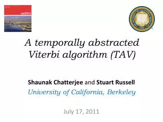
A temporally abstracted Viterbi algorithm (TAV)
650 likes | 873 Vues
A temporally abstracted Viterbi algorithm (TAV). Shaunak Chatterjee and Stuart Russell University of California, Berkeley July 17, 2011. Earth’s history – A timescale view. Widely varying timescales are pervasive in data Planning, simulation & state estimation

A temporally abstracted Viterbi algorithm (TAV)
E N D
Presentation Transcript
A temporally abstracted Viterbi algorithm (TAV) ShaunakChatterjeeand Stuart Russell University of California, Berkeley July 17, 2011
Earth’s history – A timescale view • Widely varying timescales are pervasive in data • Planning, simulation & state estimation • More efficient if timescale information is cleverly exploited 4.5Ga 1Ma 10000 yrs 600 yrs 1 yr 2 days 1 min
Images: berkeley.edu, wikipedia, food.com Where is Shaunak? Monday Tuesday Wednesday Thursday Friday Saturday Sunday Berkeley Berkeley Philadelphia Barcelona Barcelona Barcelona Barcelona Burger Cheese steak Paella Gazpacho Tapas Gazpacho Burger
State time trellis Berkeley Philadelphia Montreal Toronto Barcelona Madrid Paris Marseille t=1 t=2 t=3 t=4 t=5 t=6
The Viterbi algorithm – Viterbi, 1967 1 Berkeley 2 Philadelphia 3 Montreal 3 Toronto 4 Barcelona 4 Madrid 4 Paris 4 Marseille t=1 t=2 t=3 t=4 t=5 t=6
The Viterbi algorithm – Viterbi, 1967 1 3 Berkeley 2 4 Philadelphia 3 4 Montreal 3 4 Toronto 4 6 Barcelona 4 6 Madrid 4 8 Paris 4 8 Marseille t=1 t=2 t=3 t=4 t=5 t=6
The Viterbi algorithm – Viterbi, 1967 1 3 10 Berkeley 2 4 7 Philadelphia 3 4 15 Montreal 3 4 15 Toronto 4 6 17 Barcelona 4 6 18 Madrid 4 8 15 Paris 4 8 18 Marseille t=1 t=2 t=3 t=4 t=5 t=6
The Viterbi algorithm – Viterbi, 1967 1 3 10 13 Berkeley 2 4 7 13 Philadelphia 3 4 15 15 Montreal 3 4 15 15 Toronto 4 6 17 10 Barcelona 4 6 18 11 Madrid 4 8 15 13 Paris 4 8 18 15 Marseille t=1 t=2 t=3 t=4 t=5 t=6
The Viterbi algorithm – Viterbi, 1967 1 3 10 13 14 15 Berkeley 2 4 7 13 15 16 Philadelphia 3 4 15 15 16 17 Montreal 3 4 15 15 17 18 Toronto 4 6 17 10 11 12 Barcelona 4 6 18 11 12 13 Madrid 4 8 15 13 14 15 Paris 4 8 18 15 15 16 Marseille t=1 t=2 t=3 t=4 t=5 t=6
The Viterbi algorithm – Viterbi, 1967 1 3 10 13 14 15 Berkeley 2 4 7 13 15 16 Philadelphia 3 4 15 15 16 17 Montreal 3 4 15 15 17 18 Toronto 4 6 17 10 10 11 12 Barcelona 4 6 18 11 12 13 Madrid 4 8 15 13 14 15 Paris 4 8 18 15 15 16 Marseille t=1 t=2 t=3 t=4 t=5 t=6
The Viterbi algorithm – Viterbi, 1967 • O(N2T) by using dynamic programming • NT possible state sequences • Used in signal decoding, speech recognition, parsing and many other applications • For large N and T, this cost could be quite prohibitive • Every possible transition is considered • In some cases, many of these transitions are very unlikely to feature in the optimal path
Abstraction Berkeley U.S.A. Philly North America Montreal Canada Toronto Barcelona Spain Madrid Europe Paris France Marseille t=1 t=2 t=3 t=4 t=5 t=6
Coarse-to-fine dynamic programming (CFDP) – Raphael, 2001 Berkeley Philly Montreal Toronto Barcelona Madrid Paris Marseille t = 1 t = 2 t = 3 t = 4 t = 5 t = 6
CFDP • Step 1: Find the most likely sequence in the current state-time trellis
Coarse-to-fine dynamic programming (CFDP) – Raphael, 2001 Berkeley Philly Montreal Toronto Barcelona Madrid Paris Marseille t = 1 t = 2 t = 3 t = 4 t = 5 t = 6
CFDP • Step 1: Find the most likely sequence in the current state-time trellis • Step 2: Refine along the most likely sequence
CFDP Refinement • Node-based refinement Spain Europe France Node Refinement N.America N.America
Coarse-to-fine dynamic programming (CFDP) – Raphael, 2001 Berkeley Philly Montreal Toronto Barcelona Madrid Paris Marseille t = 1 t = 2 t = 3 t = 4 t = 5 t = 6
Coarse-to-fine dynamic programming (CFDP) – Raphael, 2001 Berkeley Philly Montreal Toronto Barcelona Madrid Paris Marseille t = 1 t = 2 t = 3 t = 4 t = 5 t = 6
CFDP • Step 1: Find the most likely sequence in the current state-time trellis • Step 2: Refine along the most likely sequence • Step 3: Go to step 1 if step 2 performed any refinement; else terminate
Coarse-to-fine dynamic programming (CFDP) – Raphael, 2001 Berkeley Philly Montreal Toronto Barcelona Madrid Paris Marseille t = 1 t = 2 t = 3 t = 4 t = 5 t = 6
Coarse-to-fine dynamic programming (CFDP) – Raphael, 2001 Berkeley Philly Montreal Toronto Barcelona Madrid Paris Marseille t = 1 t = 2 t = 3 t = 4 t = 5 t = 6
Coarse-to-fine dynamic programming (CFDP) – Raphael, 2001 Berkeley Philly Montreal Toronto Barcelona Madrid Paris Marseille t = 1 t = 2 t = 3 t = 4 t = 5 t = 6
Coarse-to-fine dynamic programming (CFDP) – Raphael, 2001 Berkeley Philly Montreal Toronto Barcelona Madrid Paris Marseille t = 1 t = 2 t = 3 t = 4 t = 5 t = 6
Coarse-to-fine dynamic programming (CFDP) – Raphael, 2001 Berkeley Philly Montreal Toronto Barcelona Madrid Paris Marseille t = 1 t = 2 t = 3 t = 4 t = 5 t = 6
Coarse-to-fine dynamic programming (CFDP) – Raphael, 2001 Berkeley Philly Montreal Toronto Barcelona Madrid Paris Marseille t = 1 t = 2 t = 3 t = 4 t = 5 t = 6
Cost bounds for abstract links • Cost of an abstract link should be a lower bound of the link refinements it encapsulates • Standard heuristic admissibility argument Correctness
Coarse-to-fine dynamic programming (CFDP) – Raphael, 2001 Berkeley Philly Montreal Toronto Barcelona Madrid Paris Marseille t = 1 t = 2 t = 3 t = 4 t = 5 t = 6
Analyzing CFDP • Great when large portions of the state-time trellis are very unlikely • Leading to fewer refinements • An appropriate abstraction hierarchy is required
An actual state trajectory Europe trip Sardinia Venice Milan Interlaken India trip Los Angeles road trip Yosemite road trip San Francisco Berkeley Stanford Jan May Sep Dec
Persistence a.k.a. Timescales Europe trip Sardinia Venice Milan Interlaken India trip Los Angeles road trip Yosemite road trip San Francisco Berkeley Stanford Jan May Sep Dec
A set of really good paths • Set 1: All paths within California for the entire month of April • Set 2: All paths that visit California and at least one other state in April • Cost(PathsApril-in-California) < Cost(PathsApril-in-1+-states) • |PathsApril-in-California | << | PathsApril-in-1+-states| • An abstraction scheme which can distinguish between these two sets of paths!
Temporally abstract link • Each link encapsulates a set of paths at the specified abstraction level over a temporal interval [T1,T2] • Just specifying start and end points is pointless! Europe Europe N.America N.America T2 T1
Links Europe Europe Direct links Paths that stay within N. America for the entire interval [T1,T2] N.America N.America T2 T1
Links Europe Europe Cross links Paths that start in Europe at T1 and end in N. America at T2 N.America N.America T2 T1
Links Europe Europe Re-entry links Paths that start and end in N. America at T1 and T2 respectively, but leave N.Americaat least once in that interval N.America N.America T2 T1
Link Refinement • No longer refining nodes! • Two types of refinement • Direct links undergo spatial refinement • Cross and re-entry links undergo temporal refinement
Europe Europe Europe Europe Spatial Refinement N.America N.America N.America N.America T1 T2 T1 T2 U.S.A. U.S.A. Canada Canada
Europe Europe Europe Europe Europe Temporal Refinement N.America N.America N.America N.America N.America T2 T1 T2 T1 T’
TAV algorithm • Identical to CFDP in structure • Step 1: Find the most likely sequence in the current state-time trellis • Step 2: Refine along the most likely sequence • Link refinement instead of node refinement • Step 3: Go to step 1 if step 2 performed any refinement; else terminate
TAV example Europe Europe N.America N.America 0 T