Download

1 / 57
630 likes | 868 Vues
Gravimeters for seismological broadband monitoring: Earth’s free oscillations. Michel Van Camp Royal Observatory of Belgium. Fundamental. 1 st Harmonic. 2 nd Harmonic. 3 rd Harmonic. What is a free oscillation?. x. L. etc. Free oscillation = stationary wave

E N D
Gravimeters for seismological broadband monitoring: Earth’s free oscillations Michel Van Camp Royal Observatory of Belgium
Fundamental 1st Harmonic 2nd Harmonic 3rd Harmonic What is a free oscillation? x L etc. Free oscillation = stationary wave • Interference of two counter propagating waves (see e.g. http://www2.biglobe.ne.jp/~norimari/science/JavaEd/e-wave4.html)
Seismic normal modes Few hours after the earthquake (0S20) Few minutes after the earthquake Constructive interferences free oscillations (or stationary waves) Periods < 54 min, amplitudes < 1 mm Observable months after great earthquakes (e.g. Sumatra, Dec 2004)
Travelling surface waves Richard Aster, New Mexico Institute of Mining and Technology http://www.iris.iris.edu/sumatra/
Historic First theories: First mathematical formulations for a steel sphere: Lamb, 1882: 78 min Love, 1911 : Earth steel sphere + gravitation: eigen period = 60 minutes First Observations: • Potsdam, 1889: first teleseism (Japan): waves can travel the whole Earth. • Isabella (California) 1952 : Kamchatka earthquake (Mw=9.0). Attempt to identify a « mode » of 57 minutes. Wrong but reawake interest. • Isabella (California) 22 may 1960: Chile earthquake (Mw = 9.5): numerous modes are identified • Alaska 1964 earthquake (Mw = 9.2) • Columbia 1970: deep earthquake (650 km): overtones IDA Network
On the sphere… Vibrating string: On the sphere: Surface eigenfunction Radial eigenfunction n = radial order n = 0 : fundamental n > 0 : overtones l, m = surface orders l = angular order -l < m < l = azimuthal order
Why studying normal modes? nAml : excitation amplitude from d one can have info on the source if all nyl and xml known Conversely: from A one can predict d : modes form the basis vectors, their combination describe the displacement (synthetic sismograms)
Why studying normal modes ? Frequencies of the eigen modes depend on : • Theshape ofthe Earth • and its density, (resistance to acceleration) shear modulus, (resistance to a change of shape) compressibility modulus (resistance to a change of volume).
Toroidal and spheroidal Using spherical harmonics (base on a spherical surface), we can separate the displacements into Toroidal (torsional) and spheroidal modes (as done with SH and P/SV waves): T : Surface eigenfunction Radial eigenfunction S :
Horizontal components (tangential) et vertical (radial) • No simple relationship between n and nodal spheres Characteristics of the modes Spheroidal modes nSml : Toroidal modes nTml: • No radial component: tangential only, normal to the radius: motion confined to the surface of n concentric spheres inside the Earth. • Changes in the shape, not of volume Not observable using a gravimeter (but…) • Do not exist in a fluid: so only in the mantle (and the inner core?) 0S2 is the longest (“fundamental”) Affect the whole Earth (even into the fluid outer core !)
n, l, m … S : n : no direct relationship with nodes with depth l : # nodal planes in latitude m : # nodal planes in longitude ! Max nodal planes = l 0S02 T : n : nodal planes with depth l : # nodal planes in latitude m : # nodal planes in longitude ! Max nodal planes = l - 1 0T03
Spheroidal normal modes: examples: ... ... ... 0S2: « football » mode (Fundamental, 53.9 minutes) 0S3: (25.7 minutes) 0S29: (4.5 minutes) 0S0 : « balloon » or « breathing » : radial only (20.5 minutes) Rem: 0S1= translation 0S29 from: http://wwwsoc.nii.ac.jp/geod-soc/web-text/part3/nawa/nawa-1_files/Fig1.jpg Animation 0S0/3 from Lucien Saviot http://www.u-bourgogne.fr/REACTIVITE/manapi/saviot/deform/ Animation 0S2 from Hein Haak http://www.knmi.nl/kenniscentrum/eigentrillingen-sumatra.html
Toroidal normal modes: examples: 0T3 (28.4 minutes) 1T2 (12.6 minutes) 0T2: «twisting» mode (44.2 minutes, observed in 1989 with an extensometer) Rem: 0T1= rotation 0T0= not existing Animation from Hein Haak http://www.knmi.nl/kenniscentrum/eigentrillingen-sumatra.html Animation from Lucien Saviot http://www.u-bourgogne.fr/REACTIVITE/manapi/saviot/deform/
Solidity demonstrated by normal modes (1971) • Differential rotation of the inner core ? Anisotropy (e.g. crystal of iron aligned with rotation)? Geophysics and normal modes Solid mantle Fluid outer core (1906) Solid inner core (1936) Shadow zone
shear energy density compressional energy density Eigenfunctions Ruedi Widmer’s home page: http://www-gpi.physik.uni-karlsruhe.de/pub/widmer/Modes/modes.html One of the modes used in 1971 to infer the solidity of the inner core: Part of the shear and compressional energy in the inner core Today, also confirmed by more modes and by measuring the elusive PKJKP phases
shear energy density compressional energy density Eigenfunctions : 0Sl Equivalent to surface Rayleigh waves l > 20: outer mantle l < 20: whole mantle Ruedi Widmer’s home page: http://www-gpi.physik.uni-karlsruhe.de/pub/widmer/Modes/modes.html
shear energy density compressional energy density Eigenfunctions : S vs. T T in the mantle only ! S can affect the whole Earth (esp. overtones) n = 10 nodal lines Ruedi Widmer’s home page: http://www-gpi.physik.uni-karlsruhe.de/pub/widmer/Modes/modes.html Deep earthquakes excite modes whose eigen functions are large at that depth
www.advalytix.de/ pics/SAWRAiGH.gif Eigenfunctions : 0Sl and 0Tl 0S equivalent to interfering surface Rayleigh waves 0T equivalent to interfering surface Love waves http://www.eas.purdue.edu/~braile/edumod/waves/Lwave.htm
«balloon» mode: T = 20.5 min. Frequency ~ 0.001 Hertz Do 256 Hertz T= 0.004 s 18 X Music and seismic normal modes
The great Sumatra-Andaman Earthquake ? http://www.iris.iris.edu/sumatra/
300 km The great Sumatra-Andaman Earthquake 1300 km
0S0 0S3 Sumatra Earthquake: spectrum Membach, SG C021, 20041226 08h00-20041231 00h00 0S4 0S2 1S2 0T2 0T4 2S1 0T3
Sumatra Earthquake: time domain Membach, SG C021, 20041226 - 20050430 Q factor 5327 Q factor 500 M. Van Camp http://www.iris.iris.edu/sumatra/
Splitting If SNREI (Solid Not Rotating Earth Isotropic) Earth : Degeneracy: for n and l, same frequency for –l < m < l For each m = one singlet. The 2m+1 group of singlets = multiplet No more degeneracy if no more spherical symmetry : Coriolis Ellipticity • 3D Different frequencies and eigenfunctions for each l, m
Waves from pole to polerun a shorter path (67 km)than along the equator Waves slowed down (or accelerated) by heterogeneities Splitting Waves in the direction of rotation travel faster • Rotation (Coriolis) • Ellipticity • 3D
Splitting Coriolis Ellipticity 3D Animation 0S2 from Hein Haak http://www.knmi.nl/kenniscentrum/eigentrillingen-sumatra.html
Splitting: Sumatra 2004 Membach SG-C021 0S2 Multiplets m=-2, -1, 0, 1, 2 “Zeeman effect” M. Van Camp http://www.iris.iris.edu/sumatra/
Coupling: Balleny 1998 In an elliptic rotating heterogeneous Earth: Mode splitting and coupling : the modes no more orthogonal An eigenfunction can contain perturbation from the eigengfunctions of neighbouring modes e.g. T can present a vertical component or Different modes at the same frequency w Displacement in SNREI Coriolis force
300-500 s surface waves http://www.gps.caltech.edu/%7Ejichen/Earthquake/2004/aceh/aceh.html Modes and Magnitude Time after beginning of the rupture: 00:11 8.0 (MW) P-waves 7 stations 00:45 8.5 (MW) P-waves 25 stations 01:15 8.5 (MW) Surface waves 157 stations 04:20 8.9 (MW) Surface waves (automatic) 19:03 9.0 (MW) Surface waves (revised) Jan. 2005 9.3 (MW) Free oscillations April 2005 9.2 (MW) GPS displacements
From aftershocks, free oscillations, GPS, … Rupture zone as determined using 300-500 surface waves Seth Stein and Emile Okal Calculated vs. observed http://www.ipgp.jussieu.fr/~lacassin/Sumatra/After/AfterNEIC-ALL.gif Modes and Magnitude
Modes and Magnitude SG C021 Membach, same duration: Sumatra 2004: Mw = 9.1-9.3 Peru 2001: Mw = 8.1 nm/s²
Undertones Oscillations Restoring force If rigidity restoring force period Seismic modes :restoring force (Elasticity, molecular cohesion) proportional with: • Shear modulus • Incompressibility • Density Sub-seismic modes (or « undertones »): m, w << restoring force proportional to: • Archimedean force : gravity waves • Coriolis force : inertial waves • Lorenz force : hydro magnetic or Alvèn waves • Magnetic Archimedean Coriolis : MAC waves
Controlled by the density jump between the inner and outer core, and the Archimedean force of the fluid core Slichter mode (triplet) (pointed out in 1961) : 1S1 • Translation of the solid inner core in the liquid outer core (1S1, period ~ 4-8 h)
Information on the stratification of the outer core Core modes • Oscillations in the fluid outer core (periods in the tidal band (?)
Undertones Normal modes of a rotating elliptic Earth Nearly Diurnal Free Wobble (NDFW) Chandler (~ 435 d)
NDFW 1.30 Y1 j1 1.20 • Nearly Diurnal Free Wobble (432 days in the Celestial frame = Free Core Nutation) d P1 K1 1.10 1.00 -0.99 -1.00 -1.01 Fréquence (cycles par jour) Observing the NDFW / FCN is thus very useful to measure the CMB flattening and to obtain information about the dissipation effect at this interface. Fortunately, the eigenfrequency of the NDFW is located within the tidal band and induces a perturbation of diurnal tides (Unfortunately the amplitude of Y1 is weak!). In the space frame, the FCN is measured by the Very Long Baseline Interferometry (VLBI). Non-Seismic proof of the fluidity of the outer core.
Chandler wobble (« polar motion ») (1891) This motion, due to the dynamic flattening of the Earth, appears when the rotation axis does not coincide anymore with the polar main axe of inertia. Without any external torque, the total angular momentum remains constant in magnitude and direction, but the Earth twists so that related to its surface, the instantaneous rotation axis moves around the polar main inertia axis. Period : 435 days (~14 months)(Chandler 1891) – 305 days if the Earth was rigid (Euler) Most probably excited by atmospheric forcing
Hydrology Polar motion, tectonics semi-diurnal Fortnightly monthly diurnal Tidal band ter-diurnal Microseism Surface waves quart-diurnal Seismic normal modes Induced by the atmosphere (« humming ») NDFW Slichter triplet Liquid outer core modes 6 h (?) Spectrum of the ground acceleration (T > 1 s) 1000 nm/s² Undertones 100 nm/s² 10 nm/s² 1 nm/s² 0.1 nm/s² 0.01 nm/s² 12 h 1d 14 d 1 month 1 s 10 s 100 s 1 h 1 yr 435 d Period
Observing normal modes Extensometres (Isabella, 1960) Long period seismometers • Spring and superconducting gravimeters !!! Not able to monitor toroidal modes (but…)
How measuring an earthquake ? inertial pendulum (same idea since 130 years !) Seismometer Seismogram Seismograph @ 10 km: M = 3 2 µm M = 5 0.2 mm
Different design of seismometers Leaf spring LaCoste Spring Bifilar (Zöllner) Inverted pendulum Garden gate
Principle of the superconducting gravimeter g g Superconducting gravimeter (magnetic levitation) Spring gravimeter mvc
Superconducting gravimeter Advantage: stable calibration factor (phase [<0.1 s] and amplitude [0.1 %]) Sumatra 2004: some seismometers suffer 5 to 10 % deviation (Park et al., Science, 2005) 10 % MW = 8.4 (largest event between 1965 and 2001) !!!
STS-1 Vertical Leaf spring Seismic mass (m) Boom g Hinge
STS-1 Horizontal Garden gate suspension Allows us to measure Toroidal AND Spheroidal modes
Newtonian effects : -4 nm/s²/hPa Loading : +1 nm/s²/hPa + local deformations Atmospheric effects (also affecting Earth tide analysis) (+ buoyancy)
Spectra after correction of the barometric effect Balleny Islands 1998, Mw=8.1
“International Deployment of Accelerometers” (Cecil and IDA Green) Late ’60ies: First idea after a LaCoste gravimeter provided nice data The original network 1975-1995 was a global network of digitally recorded La Coste gravimeters They could provide valuable constraints on earth structure and earthquake mechanisms, but a shortage of data limited further progress. During the same period, low-noise feedback seismometers were developed that allowed such data to be obtained from relatively small (and hence frequent) earthquakes. A complete description of the IDA network can be found in Eos (1986, 67 (16)) C. & I. Green
Evolution of the acquisition systems used by the IDA network Presently: 1 accelerometer + BB seismometer (STS-1, Güralp)