Computational Modeling of CpG Islands and Methylation Effects in Genomic DNA
This study explores the role of methylation in gene silencing and cell differentiation, focusing on CpG islands within DNA sequences. CpG islands, areas of high frequency of CpG dinucleotides, are often found near gene promoters and play a crucial role in gene regulation. By using computational methods, we model CpG islands, allowing us to estimate parameters and transition probabilities between methylated and unmethylated states. We also address challenges such as parameter adjustment in newly sequenced genomes where CpG island data is scarce, applying learning algorithms to refine our models based on available genomic data.

Computational Modeling of CpG Islands and Methylation Effects in Genomic DNA
E N D
Presentation Transcript
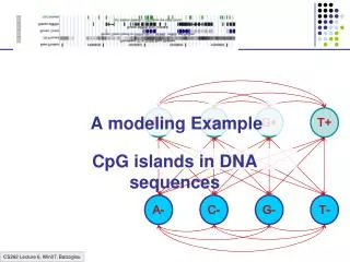
A+ C+ G+ T+ A- C- G- T- A modeling Example CpG islands in DNA sequences
Methylation & Silencing • One way cells differentiate is methylation • Addition of CH3 in C-nucleotides • Silences genes in region • CG (denoted CpG) often mutates to TG, when methylated • In each cell, one copy of X is silenced, methylation plays role • Methylation is inherited during cell division
Example: CpG Islands CpG nucleotides in the genome are frequently methylated (Write CpG not to confuse with CG base pair) C methyl-C T Methylation often suppressed around genes, promoters CpG islands
Example: CpG Islands • In CpG islands, • CG is more frequent • Other pairs (AA, AG, AT…) have different frequencies Question: Detect CpG islands computationally
A model of CpG Islands – (1) Architecture A+ C+ G+ T+ CpG Island A- C- G- T- Not CpG Island
A model of CpG Islands – (2) Transitions How do we estimate parameters of the model? Emission probabilities: 1/0 • Transition probabilities within CpG islands Established from known CpG islands (Training Set) • Transition probabilities within other regions Established from known non-CpG islands (Training Set) Note: these transitions out of each state add up to one—no room for transitions between (+) and (-) states = 1 = 1 = 1 = 1 = 1 = 1 = 1 = 1
Log Likehoods—Telling “CpG Island” from “Non-CpG Island” Another way to see effects of transitions: Log likelihoods L(u, v) = log[ P(uv | + ) / P(uv | -) ] Given a region x = x1…xN A quick-&-dirty way to decide whether entire x is CpG P(x is CpG) > P(x is not CpG) i L(xi, xi+1) > 0
A model of CpG Islands – (2) Transitions • What about transitions between (+) and (-) states? • They affect • Avg. length of CpG island • Avg. separation between two CpG islands 1-p Length distribution of region X: P[lX = 1] = 1-p P[lX = 2] = p(1-p) … P[lX= k] = pk-1(1-p) E[lX] = 1/(1-p) Geometric distribution, with mean 1/(1-p) X Y p q 1-q
What if a new genome comes? • We just sequenced the porcupine genome • We know CpG islands play the same role in this genome • However, we have no known CpG islands for porcupines • We suspect the frequency and characteristics of CpG islands are quite different in porcupines How do we adjust the parameters in our model? LEARNING
Problem 3: Learning Re-estimate the parameters of the model based on training data
Two learning scenarios • Estimation when the “right answer” is known Examples: GIVEN: a genomic region x = x1…x1,000,000 where we have good (experimental) annotations of the CpG islands GIVEN: the casino player allows us to observe him one evening, as he changes dice and produces 10,000 rolls • Estimation when the “right answer” is unknown Examples: GIVEN: the porcupine genome; we don’t know how frequent are the CpG islands there, neither do we know their composition GIVEN: 10,000 rolls of the casino player, but we don’t see when he changes dice QUESTION: Update the parameters of the model to maximize P(x|)
1. When the right answer is known Given x = x1…xN for which the true = 1…N is known, Define: Akl = # times kl transition occurs in Ek(b) = # times state k in emits b in x We can show that the maximum likelihood parameters (maximize P(x|)) are: Akl Ek(b) akl = ––––– ek(b) = ––––––– i AkicEk(c)
1. When the right answer is known Intuition: When we know the underlying states, Best estimate is the normalized frequency of transitions & emissions that occur in the training data Drawback: Given little data, there may be overfitting: P(x|) is maximized, but is unreasonable 0 probabilities – BAD Example: Given 10 casino rolls, we observe x = 2, 1, 5, 6, 1, 2, 3, 6, 2, 3 = F, F, F, F, F, F, F, F, F, F Then: aFF = 1; aFL = 0 eF(1) = eF(3) = .2; eF(2) = .3; eF(4) = 0; eF(5) = eF(6) = .1
Pseudocounts Solution for small training sets: Add pseudocounts Akl = # times kl transition occurs in + rkl Ek(b) = # times state k in emits b in x + rk(b) rkl, rk(b) are pseudocounts representing our prior belief Larger pseudocounts Strong priof belief Small pseudocounts ( < 1): just to avoid 0 probabilities
2. When the right answer is unknown We don’t know the true Akl, Ek(b) Idea: • We estimate our “best guess” on what Akl, Ek(b) are • Or, we start with random / uniform values • We update the parameters of the model, based on our guess • We repeat
2. When the right answer is unknown Starting with our best guess of a model M, parameters : Given x = x1…xN for which the true = 1…N is unknown, We can get to a provably more likely parameter set i.e., that increases the probability P(x | ) Principle: EXPECTATION MAXIMIZATION • Estimate Akl, Ek(b) in the training data • Update according to Akl, Ek(b) • Repeat 1 & 2, until convergence
Estimating new parameters To estimate Akl: (assume “|CURRENT”, in all formulas below) At each position i of sequence x, find probability transition kl is used: P(i = k, i+1 = l | x) = [1/P(x)] P(i = k, i+1 = l, x1…xN) = Q/P(x) where Q = P(x1…xi, i = k, i+1 = l, xi+1…xN) = = P(i+1 = l, xi+1…xN | i = k) P(x1…xi, i = k) = = P(i+1 = l, xi+1xi+2…xN | i = k) fk(i) = = P(xi+2…xN | i+1 = l) P(xi+1 | i+1 = l) P(i+1 = l | i = k) fk(i) = = bl(i+1) el(xi+1) akl fk(i) fk(i) akl el(xi+1) bl(i+1) So: P(i = k, i+1 = l | x, ) = –––––––––––––––––– P(x | CURRENT)
Estimating new parameters • So, Akl is the E[# times transition kl, given current ] fk(i) akl el(xi+1) bl(i+1) Akl = i P(i = k, i+1 = l | x, ) = i ––––––––––––––––– P(x | ) • Similarly, Ek(b) = [1/P(x | )]{i | xi = b} fk(i) bk(i) fk(i) bl(i+1) akl k l xi+2………xN x1………xi-1 el(xi+1) xi xi+1
The Baum-Welch Algorithm Initialization: Pick the best-guess for model parameters (or arbitrary) Iteration: • Forward • Backward • Calculate Akl, Ek(b), given CURRENT • Calculate new model parameters NEW : akl, ek(b) • Calculate new log-likelihood P(x | NEW) GUARANTEED TO BE HIGHER BY EXPECTATION-MAXIMIZATION Until P(x | ) does not change much
The Baum-Welch Algorithm Time Complexity: # iterations O(K2N) • Guaranteed to increase the log likelihood P(x | ) • Not guaranteed to find globally best parameters Converges to local optimum, depending on initial conditions • Too many parameters / too large model: Overtraining
Alternative: Viterbi Training Initialization: Same Iteration: • Perform Viterbi, to find * • Calculate Akl, Ek(b) according to * + pseudocounts • Calculate the new parameters akl, ek(b) Until convergence Notes: • Not guaranteed to increase P(x | ) • Guaranteed to increase P(x | , *) • In general, worse performance than Baum-Welch
Conditional Random Fields A brief description of a relatively new kind of graphical model
1 1 1 1 … 2 2 2 2 … … … … … K K K K … Let’s look at an HMM again 1 Why are HMMs convenient to use? • Because we can do dynamic programming with them! • “Best” state sequence for 1…i interacts with “best” sequence for i+1…N using K2 arrows Vl(i+1) = el(i+1) maxk Vk(i) akl = maxk( Vk(i) + [ e(l, i+1) + a(k, l) ] ) (where e(.,.) and a(.,.) are logs) • Total likelihood of all state sequences for 1…i+1 can be calculated from total likelihood for 1…i by only summing up K2 arrows 2 2 K x1 x2 x3 xN
1 1 1 1 … 2 2 2 2 … … … … … K K K K … Let’s look at an HMM again 1 • Some shortcomings of HMMs • Can’t model state duration • Solution: explicit duration models (Semi-Markov HMMs) • Unfortunately, state i cannot “look” at any letter other than xi! • Strong independence assumption: P(i | x1…xi-1, 1…i-1) = P(i | i-1) 2 2 K x1 x2 x3 xN
1 1 1 1 … 2 2 2 2 … … … … … K K K K … Let’s look at an HMM again 1 • Another way to put this, features used in objective function P(x, ): • akl, ek(b), where b • At position i: all K2akl features, and all K el(xi) features play a role • OK forget probabilistic interpretation for a moment • “Given that prev. state is k, current state is l, how much is current score?” • Vl(i) = Vk(i – 1) + (a(k, l) + e(l, i)) = Vk(i – 1) + g(k, l, xi) • Let’s generalize g!!! Vk(i – 1) + g(k, l, x, i) 2 2 K x1 x2 x3 xN
“Features” that depend on many pos. in x i-1 i • What do we put in g(k, l, x, i)? • The “higher” g(k, l, x, i), the more we like going from k to l at position i • Richer models using this additional power • Examples • Casino player looks at previous 100 pos’ns; if > 50 6s, he likes to go to Fair g(Loaded, Fair, x, i) += 1[xi-100, …, xi-1 has > 50 6s] wDON’T_GET_CAUGHT • Genes are close to CpG islands; for any state k, g(k, exon, x, i) += 1[xi-1000, …, xi+1000 has > 1/16 CpG] wCG_RICH_REGION x7 x8 x9 x10 x1 x2 x3 x4 x5 x6
“Features” that depend on many pos. in x x7 x8 x9 x10 x1 x2 x3 x4 x5 x6 Conditional Random Fields—Features • Define a set of features that you think are important • All features should be functions of current state, previous state, x, and position i • Example: • Old features: transition kl, emission b from state k • Plus new features: prev 100 letters have 50 6s • Number the features 1…n: f1(k, l, x, i), …, fn(k, l, x, i) • features are indicator true/false variables • Find appropriate weights w1,…, wn for when each feature is true • weights are the parameters of the model • Let’s assume for now each feature has a weight wj • Then, g(k, l, x, i) = j=1…nfj(k, l, x, i) wj
“Features” that depend on many pos. in x x7 x8 x9 x10 x1 x2 x3 x4 x5 x6 Define Vk(i): Optimal score of “parsing” x1…xi and ending in state k Then, assuming Vk(i) is optimal for every k at position i, it follows that Vl(i+1) = maxk [Vk(i) + g(k, l, x, i+1)] Why? Even though at pos’n i+1 we “look” at arbitrary positions in x, we are only “affected” by the choice of ending state k Therefore, Viterbi algorithm again finds optimal (highest scoring) parse for x1…xN
1 2 3 4 5 6 … x1 x2 x3 x4 x5 x6 1 2 3 4 5 6 … x1 x2 x3 x4 x5 x6 “Features” that depend on many pos. in x • Score of a parse depends on all of x at each position • Can still do Viterbi because state i only “looks” at prev. state i-1 and the constant sequence x HMM CRF
How many parameters are there, in general? • Arbitrarily many parameters! • For example, let fj(k, l, x, i) depend on xi-5, xi-4, …, xi+5 • Then, we would have up to K | |11 parameters! • Advantage: powerful, expressive model • Example: “if there are more than 50 6’s in the last 100 rolls, but in the surrounding 18 rolls there are at most 3 6’s, this is evidence we are in Fair state” • Interpretation: casino player is afraid to be caught, so switches to Fair when he sees too many 6’s • Example: “if there are any CG-rich regions in the vicinity (window of 2000 pos) then favor predicting lots of genes in this region” • Question: how do we train these parameters?
Conditional Training • Hidden Markov Model training: • Given training sequence x, “true” parse • Maximize P(x, ) • Disadvantage: • P(x, ) = P( | x)P(x) Quantity we care about so as to get a good parse Quantity we don’t care so much about because x is always given
Conditional Training P(x, ) = P( | x)P(x) P( | x) = P(x, ) / P(x) Recall F(j, x, ) = # times feature fj occurs in (x, ) = i=1…N fj(k, l, x, i) ; count fj in x, In HMMs, let’s denote by wj the weight of jth feature: wj = log(akl) or log(ek(b)) Then, HMM: P(x, ) =exp[j=1…n wj F(j, x, )] CRF: Score(x, ) =exp[j=1…n wj F(j, x, )]
Conditional Training In HMMs, P( | x) = P(x, ) / P(x) P(x, ) =exp[j=1…n wjF(j, x, )] P(x) = exp[j=1…n wjF(j, x, )]=: Z Then, in CRF we can do the same to normalize Score(x, ) into a prob. PCRF( | x) = exp[j=1…n wjF(j, x, )]/ Z QUESTION: Why is this a probability???
Conditional Training • We need to be given a set of sequences x and “true” parses • Calculate Z by a sum-of-paths algorithm similar to HMM • We can then easily calculate P( | x) • Calculate partial derivative of P( | x) w.r.t. each parameter wj (not covered—akin to forward/backward) • Update each parameter with gradient descent! • Continue until convergence to optimal set of weights P( | x) = exp[j=1…n wjF(j, x, )]/ Z is convex!!!
Conditional Random Fields—Summary • Ability to incorporate complicated non-local feature sets • Do away with some independence assumptions of HMMs • Parsing is still equally efficient • Conditional training • Train parameters that are best for parsing, not modeling • Need labeled examples—sequences x and “true” parses (Can train on unlabeled sequences, however it is unreasonable to train too many parameters this way) • Training is significantly slower—many iterations of forward/backward