Sample size and study design
Sample size and study design. Brian Healy, PhD. Comments from last time. We did not cover confounding Too much in one class/Not enough examples/Superficial level

Sample size and study design
E N D
Presentation Transcript
Sample size and study design Brian Healy, PhD
Comments from last time • We did not cover confounding • Too much in one class/Not enough examples/Superficial level • I wanted to show one example for each type of analysis so that you can determine what your data matches. This way you can speak to a statistician knowing the basic ideas. • My hope was for you to feel confident enough to learn more about the topics relevant to you • Worked example lectures • This is not basic biostatistics • I did Teach for America
Objectives • Type II error • How to improve power? • Sample size calculation • Study design considerations
Review • Previous classes we have focused on data analysis • AFTER data collection • Hypothesis testing allowed us to determine whether there was a statistically significant: • Difference between groups • Association between two continuous factors • Association between two dichotomous factors
Example • We know that the heart rate for healthy adult is 80 beats per minute and this has an approximately normal distribution (according to my wife) • Some elite athletes, like Lance Armstrong, have lower heart rate, but it is not known if this is true on average • How could we address this question?
Experimental design • One way to do this is to collect a sample of normal controls and a sample of elite athletes and compare their mean • What test would you use? • Another way is to collect a sample of elite athletes and compare their mean to the known population mean • This is a one sample test • Null hypothesis: meanelite=80
Question • How large a sample of elite athletes should I collect? • What is the benefit of having a large sample size? • More information • More accurate estimate of the population mean • What is the disadvantage of a large sample size? • Cost • Effort required to collect • What is the “correct” sample size?
Effect of sample size • Let’s say we wanted to estimate the blood pressure of people at MGH • If we sampled 3 people, would we have a good estimate of the population mean? • How much will sample mean vary from sample to sample? • Does our estimate of the improve if we sampled 30 people? • Would the sample mean to vary more or less from sample to sample? • What about 300 people?
Simulation • http://onlinestatbook.com/stat_sim/sampling_dist/index.html • What is the shape of the distribution of sample means? • Where is the curve centered? • What happens to curve as sample size increases? • Technical: Central limit theorem
Standard error of the mean • There are two measures of spread in the data • Standard deviation: measure of spread of the individual observations • The estimate of this is the standard deviation of the observations: • Standard error: standard deviation of the sample mean • The estimate of this is the standard deviation of the observations divided by the sample size
Technical: Distribution of sample mean under the null • If we took repeated samples and calculated the sample mean, the distribution of the sample means would have a distribution Spread in distribution is based on standard error Mean of distribution=80
Type I error • We could plot the distribution of the sample means under the null before collecting data • Type I error is the probability that you reject the null given that the null is true • a = P(reject H0 | H0 is true) Notice that the shaded area is still part of the null curve, but it is in the tail of the distribution a
Hypothesis test-review • After data collection, we can calculate the p-value • If the p-value is less than the pre-specified a-level, we reject the null hypothesis
As the sample size increases, the standard error decreases • p-value is based on the standard error • As you sample size increases, the p-value decreases if the mean and standard deviation do not change • With an extremely large sample, a very small departure from the null is statistically significant • What would you think if you found the sample mean heart rate of three elite athletes was 70 beats per minute? • Do your thoughts change if you sampled 300 athletes and found the same sample mean?
How much data should we collect? • Depends on several factors: • Type I error • Type II error (power) • Difference we are trying to detect (null and alternative hypotheses) • Standard deviation • Remember this is decided BEFORE the study!!!
Type II error • Definition: when you fail to reject the null hypothesis when the alternative is in fact true (type II error) • This type of error is based on a specific alternative b=P(fail to reject the H0 | HA is true)
Power • Definition: the probability that you reject the null hypothesis given that the alternative hypothesis is true. This is what we want to happen. Power = P(reject Ho | HA is true) = 1 - b • Since this is a good thing, we want this to be high
Fail to reject H0 Reject Ho This is the population distribution under the null hypothesis The location of the curve is m0and the spread in the curve is the standard error This is the cut-off value. This is the population distribution under the alternative hypothesis m0 m1
Fail to reject H0 Reject Ho a = P(reject H0| H0 is true) m0 Power = P(reject H0| HA is true) • = P(fail to reject H0| HA is true) m1
Life is a trade off • These two errors are related • We usually assume that the type I error is 0.05 and calculate the type II error for a specific alternative • If you are want to be more strict and falsely reject the null only 1% of the time (a=0.01), the chance of a type II error increases • Sensitivity/specificity or false positive/false negative
Changing the power • Note how the power (green) increases as you increase the difference between the null and alternative hypotheses • How else do you think we could increase the power?
Another way to increase power is to increase type I error rate • Two other ways to increase power involve changing the shape of the distribution • Increasing the sample size • When the sample size increases, the curve for the sample means tightens • Decreasing the variability in the population • When there is less variability, the curve for the sample means also tightens
Example • For our study, we know that we can enroll 40 elite athletes. • We also know that the population mean is 80 beats per minute and the standard deviation is 20 • We believe the elite athletes will have a mean of 70 beats per minute • How much power would we have to detect this difference at the two-sided 0.05 level? • All this information fully defined our curves
Using STATA, we find that we have 88.5% power to detect the difference of 10 beats per minute between the groups at the two-sided 0.05 level using a one sample z-test • Question: If we were able to enroll more subjects would our power increase or decrease?
Conclusions • For a specific sample size, standard deviation, difference between the means and type I error, we can calculate the power • Changing any of the four parameters above will change the power • Some under the control of the investigator, but others are not
Sample size • Up to now we have shown how to find the power given a specific sample size, difference between the means, standard deviation and alpha level. • We can vary any four of these five factors and find the fifth. • Usually the alpha level is required to be two-sided 0.05 • How can we calculate the sample size for specific values of the remaining parameters?
Two approaches to sample size • Hypothesis testing • When you have a specific null AND alternative hypothesis in mind • Confidence interval • When you want to place an interval around an estimate
Hypothesis testing approach • State null and alternative hypothesis • Null usually pretty easy • Alternative is more difficult, but very important • State standard deviation of outcome • State desired power and alpha level • Power=0.8 • Alpha=0.05 for two-sided test • State test • Use statistical package to calculate sample size
We know the location of the null and alternative curves, but we do not know the shape because the sample size determines the shape. We need to find the sample size that will give the curves the shape so that the a level and power equal the specified values. Alpha=0.025 Power=0.8 Beta=0.2
Sample size General form of sample size calculation • Here is the general form of the normal sample size • One-sided • Two-sided Standard deviation Related to Type I error Mean under null and alternative Related to Type II error
Hypothesis testing approach • State null and alternative hypothesis • H0: m0=80 • HA: m1=70 • sd=20 • State desired power and alpha level • Power=0.8 • Alpha=0.05 for two-sided test • State test: z-test • n=31.36 n=32
Example-more complex • In a recently submitted grant, we investigated the sample size required to detect a difference between RRMS and SPMS patients in terms of levels of a marker • Preliminary data: • RRMS: mean level=0.54 +/- 0.37 • SPMS: mean level=0.94 +/- 0.42
Hypothesis testing approach • State null and alternative hypothesis • H0: meanRRMS=meanSPMS=0.54 • HA: meanRRMS=0.54, meanSPMS=0.94, Difference between groups=0.4 • sdRRMS=0.37, sdSPMS=0.42 • State desired power and alpha level • Power=0.8 • Alpha=0.05 for two-sided test • State test: t-test
Results • Use these values in statistical package • 17 samples from each group are required • Website: http://hedwig.mgh.harvard.edu/sample_size/size.html
Statistical considerations for grant “Group sample sizes of 17 and 17 achieve at least 80% power to detect a difference of -0.400 between the null hypothesis that both group means are 0.540 and the alternative hypothesis that the mean of group 2 is 0.940 with estimated group standard deviations of 0.370 and 0.420 and with a significance level (alpha) of 0.05 using a two-sided two-sample t-test.”
Technical remarks • So we have shown that we can calculate the power for a given sample size and sample size for a given power. We can also change the clinically meaningful difference if we set the sample size and power. • In many grant applications, we show the power for a variety of sample sizes and differences in the means in a table so that the grant reviewer can see that there is sufficient power to detect a range of differences with the proposed sample size.
Confidence interval approach • If we do not have a set alternative, we can choose the sample size based on how close to the truth we want to get • In particular we choose the sample size so that the confidence interval is of a certain width
Under a normal distribution, the confidence interval for a single sample mean is • We can choose the sample size to provide the specified width of the confidence interval
Conclusions • Sample size can be calculated if the power, alpha level, difference between the groups and standard deviation are specified • For more complex setting than those presented here, statisticians have worked out the sample size calculations, but still need estimates of the hypothesized difference and variability in the data
Reasons for differences between groups • Actual effect-when there is a difference between the two groups (ex. the treatment has an effect) • Chance • Bias • Confounding
Chance • When we run a study, we can only take a sample of the population. Our conclusions are based on the sample we have drawn. Just by chance, sometimes we can draw an extreme sample from the population. If we had taken a different sample, we may have drawn different conclusions. We call this sampling variability.
Note on variability • Even though your experiments are well controlled, not all subjects will behave exactly the same • This is true for almost all experiments • If all animals acted EXACTLY the same, we would only need one animal • Since one is not enough, we observe a group of mice • We call this our sample • Based on our sample, we draw a conclusion regarding the entire population
Study design considerations • Null hypothesis • Outcome variable • Explanatory variable • Sources of variability • Experimental unit • Potential correlation • Analysis plan • Sample size
Example • We start with a single group (ex. Genetically identical mice) • The group are broken into 3 groups that are treated with 3 different interventions • An outcome is measured in each individual • Questions: • What analysis should we do? • What is the effect of starting from the same population? • Do we need to account for repeated measures?
Original group Condition 1 Condition 3 Condition 2
Generalizability • Assume that we have found a difference between our exposure and control group and we have shown that this result is not likely due to chance, bias or confounding. • What does this mean for the general population? Specifically, to which group can we apply our results? • This is often based on how the sample was originally collected.
Example 2 • We want to compare the expression of a marker in patients vs. controls • Full sample size is 288 samples • Can only run 24 samples (1 plate) per day • Questions: • What types of analysis should we do? • Can we combine across the plates? • Could other confounders be important to collect?
Plate 1: 10 patients, 14 controls Estimate of difference in this plate Plate 2: 14 patients, 10 controls Estimate of difference in this plate Plate 3: 12 patients, 12 controls Estimate of difference in this plate We can test if there is a different effect in each plate by investigating the interaction