Power Functions
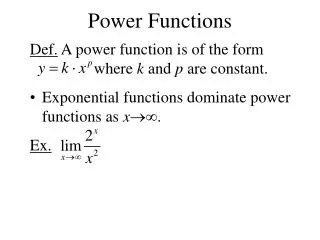
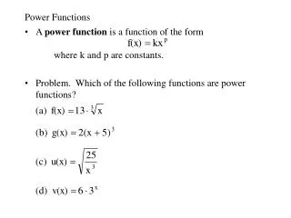
Power Functions. A power function is a function of the form where k and p are constants. Problem. Which of the following functions are power functions?. Proportionality and Power Functions. A quantity y is (directly) proportional to a power of x if

Power Functions
E N D
Presentation Transcript
Power Functions • A power function is a function of the form where k and p are constants. • Problem. Which of the following functions are power functions?
Proportionality and Power Functions • A quantity y is (directly) proportional to a power of x if • Example. The area, A of a circle is proportional to the square of its radius, r: • A quantity y is inversely proportional to xn if • Example. The weight, w, of an object is inversely proportional to the square of the object’s distance, d, from the earth’s center:
Graphs of Positive Integer Powers • Graphs of functions y = xp, where p is even and positive satisfy: • Pass through (0,0) and (1,1) and (-1,1). • Decreasing for x < 0 and increasing for x > 0. • Are symmetric about the y-axis because the functions are even. • Are concave up on every interval (U-shaped). • Larger powers dominate for x large and positive or negative. • Smaller powers dominate for x near zero.
The graphs of functions y = xp, where p is odd and positive satisfy: • Pass through (0,0) and (1,1) and (-1,-1). • Increase on every interval. • Are symmetric about the origin since the functions are odd. • Are concave down, x < 0; concave up, x > 0 (“chair”-shaped). • Larger powers dominate for x large and positive. • Smaller powers dominate for positive x near zero.
Graphs of Negative Integer Powers • The graphs of power functions with odd negative powers: all resemble the graph of y = x-1 = 1/x. • The graphs of power functions with even negative powers: all resemble the graph of y = x-2 = 1/(x2). • See the next three slides.
The graph of y = x-1: • Passes through (1,1) and (-1,-1) and does not have a y-intercept. • Is decreasing everywhere it is defined. • Is symmetric about the origin because the function is odd. • Is concave down for x < 0 and concave up for x > 0. • x-axis is horizontal asymptote; y-axis is vertical asymptote.
The graph of y = x-2: • Passes through (1,1) and (-1,1) and does not have a y-intercept. • Is increasing for x < 0 and decreasing for x > 0. • Is symmetric about the y-axis because the function is even. • Is concave up everywhere it is defined. • x-axis is horizontal asymptote; y-axis is vertical asymptote.
Comparison of graphs of y = x-1 and y = x-2 in first quadrant • As x gets large, y = x-2 approaches the x-axis more rapidly than y = x-1. • The graph of y = x-2 climbs faster than the graph of y = x-1 as x approaches zero.
Graphs of Positive Fractional Powers • The graphs of power functions with power = 1/n, n even: all resemble the graphs of y = x1/2 and y = x1/4. • The graphs of power functions with power = 1/n, n odd: all resemble the graph of y = x1/3 and y = x1/5. • See the next two slides.
The graphs of y = x1/2 and y = x1/4: • Pass through (0,0) and (1,1). • Are increasing everywhere they are defined. • Are concave down everywhere they are defined.
The graphs of y = x1/3 and y = x1/5: • Pass through (-1,-1), (0,0) and (1,1). • Are increasing everywhere they are defined. • Are concave up for x < 0 and concave down for x > 0.
Finding the formula for a power function • Problem. Find a power function g which satisfies: g(3) = 1/3 and g(1/3) = 27. Solution. We recall that a power function has the form kxp for some constants k and p. Therefore, we assume that g(x) = kxp. Taking the ratio of g(3) to g(1/3), we have We also have
Polynomial Functions • A polynomial function is a sum of power functions whose exponents are nonnegative integers. • We have previously studied quadratic functions, which are a special kind of polynomial function. We recall that a quadratic function f(x) may be written in standard form as: f(x) = ax2 + bx + c, where a, b, and c are constants, For a quadratic function, the highest power which appears in the function is 2. However, many applications require that we consider polynomials containing powers higher than 2. The next example is one such application.
An example of a polynomial with a 3rd power term • Suppose a square piece of tin measures 12 inches on each side. It is desired to make an open box from this material by cutting equal sized squares from the corners and then bending up the sides (see figure below). Find a formula for the volume of the box as a function of the length x of the side of the square cut out of each corner. The volume V(x) = x(12 – 2x)2 is found by multiplying lengthwidthheight. The formula for V(x) may be expanded to V(x) = 4x3–48x2+144x, which is a sum of power functions with nonnegative exponents. For which values of x does this formula represent the volume of the box? 12 x
A General Formula for the Family of Polynomial Functions • The general formula for the family of polynomial functions can be written as: where n is a positive integer called the degree of p and • Each member of this sum, anxn, an-1xn-1, and so on, is called a term. • The constants an, an-1, ... , a0 are called coefficients. • The term a0 is called the constant term. The highest- powered term, anxn, is called the leading term. • To write a polynomial in standard form, we arrange its terms from highest power to lowest power, going from left to right.
The Long-Run Behavior of Polynomial Functions • When viewed on a large enough scale, the graph of the polynomial looks like the graph of the power function y = anxn. This behavior is called the long-run behavior of the polynomial. • Example. Let p(x) = x2 + x. Then we have It follows that the graph of p(x) is trapped between the graph of x2 and the graph of 2x2 for x > 1. For this reason, we say that the graph of p(x) looks like the graph of x2 when viewed on a large scale.
Using the long-run behavior of a polynomial to locate zeros • The zeros of a polynomial p are the values of x for which p(x) = 0. These values are also called the x-intercepts, because they tell us where the graph of p crosses the x-axis. • Problem. Given the polynomial where q(0) = –1, is there a reason to expect a solution to the equation q(x) = 0? Solution. Since the graph of the polynomial q(x) resembles that of y = 3x6 for large (positive or negative) values of x, we know that the graph of q(x) is greater than zero for these large values of x. Since q(0) < 0 and the graph of q is smooth and unbroken, it follows that this graph must cross the x-axis at least twice.
Summary of Power and Polynomial Functions, Sections 9.1, 9.2 • Power functions were defined and properties of graphs were studied for various classes of power functions. • We discussed finding the formula for a power function when two points on its graph are given. • Polynomials were defined to be a sum of power functions: • The degree of a polynomial is the value n in the formula above. • Long-run behavior of polynomials was discussed. • Zeros of polynomials were investigated and the long-run behavior was used to show their existence in some cases.
The Short-Run Behavior of Polynomials • The shape of the graph of a polynomial depends on its degree; typical shapes are shown below. Cubic (degree = 3) Quartic (degree = 4) Quintic (degree = 5) Quadratic (degree = 2)
The long-run behavior of a polynomial is determined by its leading term. However, polynomials with the same leading term may have very different short-run behaviors. • Example. Compare the graphs of f(x) = x3 – x and g(x) = x3 + x. Note that f has three zeros while g has only one.
The Factored Form of a Polynomial • To predict the long-run behavior of a polynomial, we write it in standard form. However, to determine the zeros of a polynomial, we write it in factored form, as a product of other polynomials. Some, but not all, polynomials can be factored. • Problem. Rewrite the third-degree polynomial u(x) = x3 – x2 – 6x as a product of linear factors. Solution. By factoring out an x and then factoring the quadratic, x2 – x – 6, we rewrite u(x) as • The advantage of the factored form is that we can easily find the zeros of the polynomial using the rule:
Linear Factors of a Polynomial • Suppose p is a polynomial. If the formula for p has a linear factor, that is, a factor of the form (x – k), then p has a zero at x = k. Conversely, if p has a zero at x = k, then p has a linear factor of the form (x – k). • If a polynomial doesn’t have a zero, this doesn’t mean it can’t be factored. For example, the polynomial p(x) = x4 + 5x2 + 6 has no zeros. To see this, note that x4 and 5x2 are never negative. However, this polynomial can be factored as p(x) = (x2 + 2)(x2 + 3). The point is that a polynomial with a zero has a linear factor, and a polynomial without a zero does not.
Polynomials, zeros, and linear factors • p(k) = 0 (x – k) is a factor of polynomial p. • If p(x) = (x–3)(x+1)(x–2), name three zeros of p. k1= ?, k2= ?, k3= ?. • If another polynomial p satisfies p(1) = 0, p(5) = 0, p(–3)=0, name three linear factors of p. (x – ?), (x – ?), (x – ?).
The Number of Factors, Zeros, and Bumps • The number of linear factors is always less than or equal to the degree of a polynomial. (Do you see why?) Since each zero corresponds to a linear factor, the number of zeros is less than or equal to the degree of the polynomial. • Between any two consecutive zeros, there is a bump in the graph because it changes direction. • The above observations can be summarized by the following statement: The graph of an nth degree polynomial has at most n zeros and turns at most (n–1) times.
Multiple Zeros • If p is a polynomial with a repeated linear factor, then p has a multiple zero. • If the factor (x – k) is repeated an even number of times, the graph of y = p(x) does not cross the x-axis at x = k, but “bounces” off the x-axis there (see left below). • If the factor (x – k) is repeated an odd number of times, the graph of y = p(x) crosses the x-axis at x = k, but it looks flattened there (see right below).
An Unknown Polynomial • If we know the polynomial f whose graph is shown below has degree 4, what can we conclude about its zeros? • The graph suggests that f has a single zero at x = 1. The flattened appearance near x = -1 suggests that f has a multiple zero there. Since the graph crosses the x-axis at x = -1, we conclude the zero there is repeated an odd number of times. Since f has degree 4, there must be a triple zero at x = -1.
Finding a possible formula for a polynomial from its graph • Problem. Find a possible formula for the polynomial f which is graphed below. • Solution. Based on its long-run behavior, f is of odd degree greater than or equal to 3. The polynomial has zeros at x = -1 and x = 3. We see that x = 3 is a multiple zero of even power, because the graph “bounces off” the x-axis here. Therefore, we try the formula f(x) = k(x+1)(x–3)2, where k represents a stretch factor. The shape of the graph shows that k is negative. We read f(0) = -3 from the graph, and we use the formula to get k = -1/3.
A General Formula for the Family of Rational Functions • If r is a function that can be written as the ratio of two polynomials p and q so that then r is called a rational function. Here, it is assumed that q(x) is not the constant polynomial with value zero. • Example. The function is actually a rational function. In order to see this, we must combine the terms of f by finding a common denominator.
The Long-Run Behavior of Rational Functions • For large enough values of x (either positive or negative), the graph of the rational function r looks like the graph of a power function. If then the long-run behavior of y = r(x) is given by • Example. Suppose that then, in the long run, r(x) behaves like 2x. The Maple plot of y = r(x) is shown on the next slide.
>plot((2*x^2+1)/(x-1), x = -5..10, y = -50..50, discont =true); Note that far from the origin, the graph resembles that of y = 2x. Also note that the graph has a vertical asymptote at x = 1.
Compare and discuss the long-run behaviors of the following functions: • f(x) = • g(x) = • h(x) = • Note that none of the above functions has a vertical asymptote. Can you explain why?
Summary of Polynomial and Rational Functions, Sections 9.3, 9.4 • The number of linear factors, zeros, and bumps and their relation to the degree was discussed. • Factored form and its linear factors were used to find the zeros and analyze the short-run behavior of a polynomial. • If a multiple zero of a polynomial is repeated an even number of times, the graph of the polynomial does not cross the x-axis at the zero, but “bounces” off the x-axis there. • If a multiple zero of a polynomial is repeated an odd number of times, the graph of the polynomial crosses the x-axis at the zero, but it looks flattened there. • By analyzing long-run behavior and using the properties listed above, we were able to find a possible formula for a polynomial if its graph was given. • Rational functions r(x) are defined as the ratio of two polynomials, p(x) in the numerator, and q(x) in the denominator. • Long run behavior of r(x): y = (lead term of p(x))/(lead term of q(x)).
The short-run behavior of rational functions • The first step in analyzing the short-run behavior of a rational function where p and q are polynomials, is to factor p and q, if possible. • Example. Let As a first step in analyzing the behavior of r(x), we factor the denominator to obtain • Note that the zeros of r(x) will be the same as the zeros of the numerator, p(x), assuming that p and q have different zeros. In the example, r(x) has a zero at x = –2/3.
The vertical asymptotes of a rational function • Just as we can find the zeros of a rational function by looking at its numerator, we can find the vertical asymptotes by looking at its denominator. A rational function is large (positively or negatively) wherever its denominator is small. This means that a rational function r(x) = p(x)/q(x) has a vertical asymptote wherever q(x) is zero (assuming that p(x) and q(x) have different zeros). • Example. Again let Since the zeros of the denominator are 1 and –2, we conclude that the graph of r has vertical asymptotes at 1 and –2. Note that the zeros of the numerator and denominator are different.
The graph of a rational function • We summarize what we have learned about the graph of a rational function r(x) = p(x)/q(x), where p(x) and q(x) are polynomials with different zeros. • The long-run behavior of r is given by the ratio of the leading terms of p and q. • The zeros of r are the same as the zeros of p. • The graph of r has a verticalasymptote at each of the zeros of the denominator, q. • We can apply the above principles to help us draw the graph of a rational function. Also of interest is the y-intercept of the graph, which is found by evaluating r(0), assuming that r is defined at x = 0.
Example. The graph of Vertical Asymptote at x = –2 Horizontal Asymptote at y = 0 Vertical Asymptote at x = 1 Note that the x-intercept is –2/3 and the y-intercept is – 1.
Some rational functions are transformations of power functions • Problem. Show that the rational function r(x) = (x+3)/(x+2) is a translation of the power function f(x) = 1/x. Solution. The numerator of r may be rewritten as Upon dividing, we have Thus, the graph of y = r(x) is the graph of y = 1/x shifted two units to the left and one unit up. The graph of y = r(x) is shown below. What is the vertical asymptote? the horizontal asymptote?
Finding the formula for a rational function from its graph • For a rational function, we can read the zeros and vertical asymptotes from its graph. The zeros correspond to factors in the numerator and the vertical asymptotes correspond to factors in the denominator. • Problem. Given the graph, find a possible formula for r(x). • Solution. What is the value of k?
When p(x) and q(x) have the same zeros: holes • We have been studying rational functions r(x) = p(x)/q(x) under the assumption that p(x) and q(x) have different zeros. The following example indicates what can happen when this assumption does not hold. • Example. Let r(x) = Here, p(x) = x2 + x – 2 can be factored into (x – 1) and (x + 2) so that p(x) and q(x) have x = 1 as a common zero. If we cancel the common factor, the formula for r becomes r(x) = x + 2, x 1. Do you see why x cannot equal 1? The graph of y = r(x) is shown below: The graph has a hole at x = 1.
Comparing Power, Exponential, and Log Functions • Any positive increasing exponential eventually grows faster than any power function. • Any positive decreasing exponential eventually approaches the horizontal axis faster than any positive decreasing power function. • Any positive increasing power function eventually grows more rapidly than y = log x and y = ln x. • Futhermore, the three results stated above are not changed if one of the functions is multiplied by a positive constant. • Problem. Which of the following functions will dominate for large positive x: f(x) = 1,000,000x2 or g(x) = 0.000001ex ? Solution. Using the first and fourth bullet points above, we see that g will dominate f if x is chosen to be a sufficiently large positive number.
Summary of Polynomial and Rational Functions, Sections 9.5, 9.6 • Rational functions r(x) are defined as the ratio of two polynomials, p(x) in the numerator, and q(x) in the denominator. • The long-run behavior of r(x) is given by: • Assuming that p and q do not have common zeros, the zeros of r are the same as those of p, and the vertical asymptotes of r occur at the zeros of q. • From the graph of a rational function we can determine its formula. • If p(x) and q(x) have common zeros, the graph of y = r(x) will have “holes” at the common zeros. • We compared growth rates of powers, exponentials, and logarithms.