Efficient PCPs: Balancing Proof Size and Verifier's Running Time
340 likes | 462 Vues
This paper explores short and efficient PCPs, revisiting the study of lower and upper bounds, with a focus on coding theory, cryptography, and sublinear verification. It delves into the challenges and progress made in constructing PCPs, aiming for practical implementations and efficient verifiers. Theoretical results on blowup in proof size, query complexity, and running time are presented, emphasizing the trade-offs between efficiency and accuracy in proof verification. The paper discusses improvements in PCP constructions, particularly in reducing blowup and queries while maintaining higher efficiency. Various constructions and modifications in constructing efficient PCPs are examined in detail.

Efficient PCPs: Balancing Proof Size and Verifier's Running Time
E N D
Presentation Transcript
Short PCPs verifiable in Polylogarithmic Time Eli Ben-Sasson, TTI Chicago & Technion Oded Goldreich, Weizmann Prahladh Harsha, Microsoft Research Madhu Sudan, MIT Salil Vadhan, Harvard
h h T T x x - - e e o o r r e e m m 1 [ ( ) ] 9 L P V = [ ( ) ] ¼ 1 1 8 L P V ¼ 1 · 2 2 x ¼ r x ) = = x ¼ r x ) = ; ; 2 Proof Verification: NP to PCP V V PCP Theorem [AS, ALMSS] (deterministic verifier) (probabilistic verifier) NP Proof • Parameters: • # random coins - O(log n) • # queries - constant • proof size - polynomial Completeness: Soundness:
Study of PCPs Initiated in the works of • [BFLS] • positive result • [FGLSS] • negative result Very different emphases
Direct Motivation: Verification of Proofs Important Parameters Proof Size Verifier Running Time randomness query complexity h T x - e o r e m BFLS: Holographic proofs VL PCP Verifier
FGLSS: Inapproximability Connection • Dramatic Connection • PCPs and Inapproximability • Important Parameters • randomness • query complexity
Work since BFLS and FGLSS • Almost all latter work focused on the inapproximability connection • improving randomness and query complexity of PCPs • Very few works focused on PCP size • specifically, [PS, HS, GS, BSVW, BGHSV, BS] • No latter work considered the verifier’s running time • This paper: revisit study of efficient PCPs
Short and Efficient PCPs? • Lower Bounds • Tightness of inapproximability results wrt to running time • Upper Bounds • Future “practical implementations” of proof-verification • Coding Theory • Locally testable codes [GS, BSVW, BGHSV, BS] • Relaxed Locally Decodable Codes [BGHSV] • Cryptography • e.g.: non-blackbox techniques [Bar]
Motivation: short PCP constructions • [BFLS] Blowup in proof size: n Running time: poly log n • Recent progress in short PCP constructions • [BGHSV] Blowup: exp ((log n) )) # Queries: O(1/) • [BS] Blowup: poly log n # Queries: poly log n Can these improvements be accompanied with an efficient PCP verifier?
( ) h d E C C T E i L ( ) f f E L x - x e o r - e m n c o n g 2 ¡ x ) y a r r o m n c ) ( ) E [ 1 ] 9 P V n c x ¼ [ ] 1 1 8 P V y ¼ 1 · ; ¼ r = = ; ¼ r = ; 2 ; Sublinear Verification Sublinear running time? Not enough to read theorem ! [BFLS] Assume theorem is encoded VL Completeness: PCP Verifier Soundness: Important: # queries = sum of queries into encoded theorem + proof
h T [ ] 9 L P V ( = ) x ¼ 1 1 ± ¢ L L x - e o r e m 2 2 > ; x ¼ r ) = = x x ) ) ; ; 1 1 [ [ ( ( ) ) ] ] 8 8 P P V V x x ¼ ¼ 1 1 · · ; ; ¼ ¼ r r = = 2 2 ; ; ¼ PCP of Proximity (PCPP) [BGHSV, DR] Completeness: Soundness: V (probabilistic verifier) • # queries = sum of queries • into theorem + proof • Theorem in un-encoded format • – proximity parameter • Assignment Testers of [DR]
Our Results: Efficient BS Verifier • Theorem: Every L2 NTIME(T(n)) has a PCP of proximity with • Blowup in proof size: poly log T(n) • # queries: poly log T(n) • Running time:poly log T(n) • Corollary [efficient BS verifier]: Every L2 NP has PCPPs with blowup at most poly log n and running timepoly log n Previous Constructions required polyT(n) time
Our Results: Efficient BGHSV Verifier Previous Constructions required polyT(n) time • Theorem: Every L2 NTIME(T(n)) has a PCP of proximity with • Blowup in proof size: exp ((log T(n)) ) • # queries: O(1/ ) • Running time:poly log T(n) • Corollary [efficient BGHSV verifier]: Every L2 NP has PCPPs with blowup at most exp ((log n) ), # queries O(1/ ) and running timepoly log n
Efficient PCP Constructions • Overview of existing short PCP constructions • specifically, construction of [BS] • Why these constructions don’t give efficient PCPs? • Modifications to construction to achieve efficiency
PCP Constructions – An Overview • Algebraic Constructions of PCP (exception: combinatorial const. of [DR] ) • Step 1: reduction to “nice” coloring CSP • Step 2: arithmetization of coloring problem • Step 3: zero testing problem • Note: Step 1 required only for short PCPs. Otherwise arithmetization can be directly performed on SAT. This however blowups the proof size.
I t n s a n c e x V i t - v e r c e s Step 1: Reduction to Coloring CSP deBruijn graph + Set of Coloring Constraints on vertices • Size of graph |V|u size of instance |x| • Graph does not depend on x, depends only on |x|. • Only coloring constraints depend on x
3 f g C V C 0 1 £ o n : ! ; l C V C o : ! L 2 x v m 9 l l f l l h C V C i i i i t t t t ¡ a c o o r n g o : s a s y n g a e c o n s r a n s ! . Step 1: Reduction (Contd) Coloring Constraints encode action of NTM on instance x • C – (constant sized) of colors • Coloring Function Coloring Constraint Valid? Proof of “x2L”: Coloring Col : V!C
b d d h E B H i j i m e e r u n g r a p n : b S H F t ½ u s e h h l A H i i t t t t 2 l d s s o F c a e e F a c v e r e x v w a n e e m e n x i e j j j j H V ¼ Step 2: Arithmetization F H
h l l l l l B i w e r e - o c a p o y n o m a r u e ^ 3 3 f g C C F V F C F 0 1 9 9 l l d d l l l l l h L L F F F F £ £ i i i 2 2 ^ o o n n : : ! ! x x a a o o w w - - e e g g r r e e e e c p o o o y r n n o m g p a o y p n : o m a p : s u c , , ! ! d b f C F i l l C C H V F C t t t ; o n s a n s z e s u s e o o : o : ! ! ^ ( ( ) ( ( ( ) ) ) ( ( ) j ) ) h h h h l l ¯ 8 C B N N H i i 0 0 t t t t t t 2 ´ ´ s u a c e a p o o y n n o x m p a x q p p x s a p s e s x q x C = H 1 2 l d l F F ; ; ; ; . o w e g r e e p o y p : L ! 2 x . m 9 l l f l l h C V C i i i i t t t t ¡ a c o o r n g o : s a s y n g a e c o n s r a n s ! . Step 2: Arithmetization (Contd) • Colors • Coloring Constraint • Coloring Proof of “x2L”: Polynomials p,q :F!F
F H F F q : ! Step 3: Zero Testing • Instance: • Field F and subset HµF • Function q: F!F(specified implicitly as a table of values) • Problem: • Need to check if q is close to a low-degree polynomial that is zero on H • Two functions are close if they differ in few points
Low Degree Testing • Sub-problem of zero-testing • Instance: • Field F and subset HµF • Function q: F!F(specified implicitly as a table of values) • Problem: • Check if q is close to a low-degree polynomial. • Most technical aspect of PCP constructions • However, can be done efficiently (for this talk)
( ) Q ( ) h L Z t ¡ Z e x x = H ´ ¢ q r h H h 2 Step 3: Zero Testing (Contd) • Obs:q:F!F is a low-degree polynomial that vanishes on Hif there exists another low-degree polynomial r such that • Instance: q: F!F Proof:r:F!F • (Both specified as a table of values) • Testing Algorithm: • Check that both q and r are close to low-degree polynomials (low-degree testing) • Choose a random point x2RF, compute ZH(x ) and check that q(x) = ZH(x) ¢r(x)
3 f g C V C 0 1 £ o n : ! ; PCP Verifier • Instance: x Proof: p,q,r : F!F • Step 0: [Low Degree Testing] • Check that the functions p, q andr are close to low-degree poly. • Step 1: [Reduction to Coloring CSP] • Reduce instance x to the coloring problem. More specifically, compute the coloring constraint • Step 2: [Arithmetization] • Arithmetize the coloring constraint Con to obtain the local rule B • Check that at a random point q = B(p) is satisfied • Step 3: [Zero Testing] • Choose a random pointx2RF and compute ZH(x) • Check that p(x) = ZH(x) ¢R(x) Each of the 4 steps efficient in query complexity However, Steps 1,2 and 3 are NOT efficient in Verifier’s running time
Step 3: Zero Testing – Efficient? • Zero Testing involves computing ZH(x) • General H: Zero Testing – inefficient • ZH has |H| coefficients • Size of instance - O(|H|) • Hence, requires at least linear time • Do there exist H for which ZH(x) can be computed efficiently • YES!, if H is a subgroup of F instead of an arbitrary subset of F, then ZH is a sparse polynomial
( ) ( ) f b f h I H F G F H H i i i i 2 ( ) t t + b ¯ l d f f f L F G F S F F i i i q 2 2 2 2 t t s a s u g r o u p o c o n a n n g e x y x y e n ) e e a n e x e n s o n e o o s z e u p p o s e : s a n ! . . , ; , . h h Z i i ( ( ) ( ) ( ) ) h h f f f f l l h f b F i i t s a o m o m o r p s m + + 2 H o m o m o r p s m e x y x y o r a x y e n c a n e = . . . , , ; , d f l l e x p r e s s e a s o o w s ¡ 1 q 2 4 2 ( ) f + + + + ¢ ¢ ¢ x c x c x c x c x = 0 1 2 1 ¡ q ( ) f h l l i i i t t e a s a s p a r s e p o y n o m a r e p r e s e n a o n . . , Facts from Finite Fields • Fact 1 • Fact 2 • Hence, ZH is sparse (i.e, ZH has only log |H| coefficients). Moreover, these coeffs. Can be computed in poly log |H| time.
( ) b ¯ l d f f f L F G F S F F i i q i 2 2 t t e e a n e x e n s o n e o o s z e u p p o s e : s a n ! . ( ( ) ( ) ( ) ) h h f f f f l l h f b F i i t + + 2 o m o m o r p s m e x y x y o r a x y e n c a n e = . . , , ; , d f l l e x p r e s s e a s o o w s ¡ 1 q 2 4 2 ( ) f X + + + + ¢ ¢ ¢ x c x c c x c x = 0 1 2 1 ¡ q ( ) f h l l i i i t t e a s a s p a r s e p o y n o m a r e p r e s e n a o n . . , Fact 1: Homomorphisms are sparse Proof: • Set of homomorphisms from F to F form a vector space over F of dimension q • The functions x, x2, x4, ….., x2q-1 are homomorphisms • The functions x, x2, x4,……, x2q-1 are linearly independent Hence, any homomorphism can be expressed as a linear combination of these functions ¥
( ) ( ) f b f h I H F G F H H i i i i 2 t t + 2 2 s a s u g r o u p o c o n a n n g e x y x y e n ) . . , ; , h h Z i i s a o m o m o r p s m H . ( ) ( ) ( ) ( ) 8 Z Z Z F + 2 ´ p x y x y x y x y H H H ; ; ; Fact 2: H subgroup )ZH homomorphism Proof: • Need to show • Degree of p·|H| • If x2H or y2H, then p(x,y) = 0 • Hence, number of zeros of p is 2|H||F|-|H|2 > |H||F| • Fraction of zeros > |H|/|F| ¸ deg(p)/|F| Hence, by Schwartz-Zippel, p´ 0¥
I t n s a n c e x V i t - v e r c e s Step 1: Efficiency of Reduction deBruijn graph + Set of Coloring Constraints on vertices • Reduction involves computing coloring constraint • Con: V£C3! {0,1} • Not efficient – requires poly |x| time (each constraint needs to look at all of x)
Step 1: Succinct Coloring CSP • Need to compute constraint without looking at all of x! • Succinct description: For any node v, the coloring constraint at v can be computed in poly |v| time (by looking at only a few bits of x) • Even this does not suffice (for arithmetization): • Further require that the constraint itself can be computed very efficiently (eg., by an NC1 circuit) • Gives a new NEXP-complete problem
Step 1: Succinct Coloring CSP (Contd) • Succinct Coloring CSP: Same as before • DeBruijn graph + Coloring Constraints • Additional requirement: Coloring Constraint at each node described by an NC1 circuit and furthermore given the node v, the circuit describing constraint at node v can be computed in poly |v| time • Reduction to Succinct CSP uses reduction of TM computations to ones on oblivious TMs[PF] • Thus, Step 1 can be made efficient
^ 3 3 f g C C F V F C F 0 1 £ £ o o n n : : ! ! ; Step 2: Arithmetization – Efficient? • Arithmetization of coloring constraint • Obtained by interpolation • Time O(|V|)=O(|H|) • However, require that the arithmetization be computed in time poly log |H| • Non trivial ! • All we know is Con is a small sized (NC1) circuit when its input is viewed as a sequence of bits • Require arithmetization of Con to be small sized circuit when its inputs are now field elements and the only operations it can perform are field operations
3 f g C V C 0 1 £ o n : ! ; v v v c c c 1 2 1 2 3 m ; ; : : : ; ; ; ; Step 2: Efficient Arithmetization • Obs: The function extracting the bitvi from the field element is a homomorphismvi: F!F • Use Fact 1 (of finite fields) again: Homomorphisms are sparse polynomials • Hence, each input bit to circuit can be computed efficiently • Resulting algebraic circuit for Constraint • Degree – O(|H|) • Size – poly log |H| • Hence, efficient • The remaining circuit is arithmetized in the standard manner • AND (x,y) !x¢y (product) • NOT(x) ! (1-x)
Putting the 3 Steps together… • Plug the efficient versions of each step into PCP verifier to obtain the polylog PCP verifier • Summarizing… • Efficient versions of existing short PCP constructions