Engineering Equation Solver Tutorials Spring 2004
Engineering Equation Solver Tutorials Spring 2004. Session I Introduction to EES. By Hrishikesh Gadre Email: hgadre1@lsu.edu. Department of Mechanical Engineering Louisiana State University. Session 1 Outline. What is EES What EES can do for you Getting started with EES

Engineering Equation Solver Tutorials Spring 2004
E N D
Presentation Transcript
Engineering Equation Solver TutorialsSpring 2004 Session I Introduction to EES By Hrishikesh Gadre Email: hgadre1@lsu.edu Department of Mechanical Engineering Louisiana State University
Session 1 Outline • What is EES • What EES can do for you • Getting started with EES • Solving a thermodynamics problem. • About Windows menu.
What is EES • Engineering Equation Solver. • Solves large sets of non-linear algebraic equations. • Built-in functions for thermodynamic and transport properties. • Highly popular software in teaching courses like Thermodynamics, Heat Transfer and Fluid Mechanics.
What EES can do for you • Solve set of simultaneous algebraic equations • Can be used to solve differential and integral equations • Generate publication-quality plots. • Capable of doing linear and non-linear regression. • Check unit consistency, do optimization etc.
EES over other equation-solving programs • Automatically identifies and groups equations that must be solved simultaneously. • Provides many built-in thermodynamic and mathematical functions. • Also, allows user to enter his/her own functions
Getting started with EES • To get familiar with EES, let’s start with a simple example • Solve set of 3 equations with 3 variables simultaneously.
Starting new program in EES • Start EES • Click File menu • Click on New
Entering the equations… • You will get a blank equations window. • Equations can be entered in the same manner as for any word processor.
Formatted equations • The entered equations can be seen in the normal mathematical format. • For that, go to Windows menu, and click on Formatted Equations. • You will see Formatted Equations window like this.
Solving those equations… • To solve these equations, go to Calculate menu and click on Solve, or directly press F2. • Immediately, you will see this window before the solution window appears.. • There are few things to note about this window. • Mainly, it shows the number of blocks, into which it has divided the total equations, it also shows the time taken for the calculations.
Solution window • Here is the Solution window as it looks. • It also shows the current unit settings • And if there are any unit consistency or conversion problems.
Tables… • Now, we will see how Tables menu work in EES. • For that, we will consider first and third of our three equations. • The second equation is enclosed within {} brackets. • So, it will not be considered while calculation, which is reflected in Formatted Equation window.
Tables continued… • Go to Tables menu, select New Parametric Table • A dialog box as shown below appears, select all three variables x,y,z on left, then click Add and then OK. • Then, you get a blank table like this.
Go to Tables menu and select Alter Values. • The dialog box as shown appears. • Select ‘x’ in the left window. Input the First Value as 1, then select Last value option from drop down list and enter 20 as the last value. Then click Apply.
Solving the table • You can see column of x filled with 10 values equally spaced within 1 and 20. • Then go to Calculate menu and click Solve Table. • Enter First run as 1 and Last Run as 10 and it calculates values for y and z according to the two equations.
Plots • Go to Plots menu, click New Plot Window and select X-Y plot. • Select x as X-Axis and y as Y-Axis, and click OK.
Plots continued… • You will get a plot like this. • This plot plots the column y against column x. • Seen on the right side is the toolbar. With the Add text button on it, we can add text items on the plot.
Plot over plot • Go to Plots menu again and select Overlay Plot. • Choose x as X-Axis and z as Y-Axis and select Y2 (right Y-scale) from drop-down list.
You get a overlay plot (both plots in same window) as shown. • Here you can also see the example of adding text items on the plot. • This completes the discussion of this problem.
A Thermodynamics problem • Example 2-2 from Thermodynamics, 6/e by Wark and Richards. • A small race car (go-kart) has a mass of 200 pounds with the rider and is powered by a 3-horsepower engine. Estimate how long it would take the go-kart to reach a speed of 40 miles per hour on a level racetrack. Assume that all of the engine power can be available as mechanical power to accelerate the go-kart.
Setting the units • Go to Option menu, select Unit System. • It shows the units currently being used by EES. • Make sure the correct units are set and then proceed to solve the problem.
Equations… The main equations would be like this: • Power=3 “hp” • m_car=200 “lbm” • V_2=40 “mph” • V_1=0 “mph” • DELTAKE_car=W_mech • DELTAKE_car=m_car*(V_2^2-V_1^2)/2*convert(lbm-mph^2, ft-lbf) • W_mech=Power*DELTAt*convert(hp-s, ft-lbf)
Use of Convert function • The ‘Convert’ function provides unit conversion. • The format is convert(‘From’,‘To’), where From and To are Unit designations. • E.g. a=convert(ft,in) will give a=12 as solution.
Formatted equations • This is how Formatted Equations window will look like. • Note, here in place of the function convert, the actual conversion factor is written. • Calculate-> Solve, will solve these equations.
Variable information • If you want your final solutions to be displayed with unit, you can go to Option menu and select Variable Info. • Enter the units manually in Units column. • Also, you can set different things like initial guess, lower and upper limits and the display format of those variables.
Windows menu • The Windows menu in EES gives different windows related with the problem. • The interesting point here is worth noting. The ‘Close Window’ control merely hides the window and doesn’t actually delete it. That means, a closed window can be reopened any time by selecting it from Windows menu. • Explore different options available in the menu like Tile, Cascade etc.
Equations Window • Equation window operates much like a word processor. • Comments are enclosed in braces {} or “ ”. Comments within {} are not shown in Formatted Equations window but those in “” are shown. • Equations may be entered in any order. EES will block these equations and reorder them for efficient solution.
Formatted Equations window • This window displays the same equations as in Equations window but in a mathematical format which is easy-to-read. • Examples include DELTA is shown by the symbol • If you write a_1, it will be shown as
Residual windows • The Residual window, gives relative and absolute residual values. • In addition, it also indicates equation blocking and calculation order used by EES.
Diagram window • This window has several functions. • Basically, it gives area to display graphics and text relating to the problem, e.g. a schematic diagram to help interpret the equations. • Secondly, it can also be used to provide convenient input and output of data. • Buttons can be located on this window such as Calculate button to initiate the calculations.
Diagram window continued… • This shows the diagram window for the problem discussed. • It shows example of how diagram window can be used for input and output of information.
Recap What we have learnt today. • What is EES, its capabilities and advantages. • Getting started with EES • Solving a thermodynamics problem. • About Windows menu.
Thank You • That’s all for today…. • THANK YOU