Western Larch in NA
270 likes | 383 Vues
Understanding species distribution is critical for biodiversity conservation and ecosystem management. This article reviews the latest non-parametric habitat modeling techniques that account for complex interactions within ecological data. We discuss methods to predict habitat suitability using species occurrence data, environmental variables, and various statistical models, including Maxent and Random Forests. With an emphasis on montane frogs and Eurasian tree sparrows, we highlight the importance of modeling in the face of climate change. Moreover, we address challenges such as data uncertainty and overfitting in ecological studies.

Western Larch in NA
E N D
Presentation Transcript
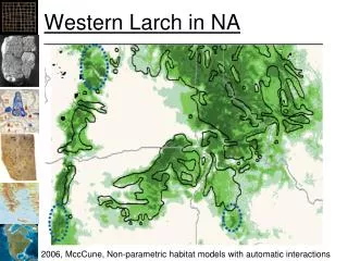
Western Larch in NA 2006, MccCune, Non-parametric habitat models with automatic interactions
2006, MccCune, Non-parametric habitat models with automatic interactions
Montane Frogs in Rainforest 2013, Marcio et al., Understanding the mechanisms underlying the distribution of microendemic montane frogs (Brachycephalus spp., Terrarana: Brachycephalidae) in the Brazilian Atlantic Rainforest
Two Approaches Occurrence/Presence Mechanistic Occurrences “Greenhouse” experiments Correlate Design Model Model Predictor Layers Generate Generate Map
Habitat Suitability Models • Find the suitable habitat for a species • Also called “Species Distribution Models” Tamarisk, NIISS.org Tree Sparrow, Herts Bird Club
Geographical Space Observed Occurrences Realized Niche/Distribution Environmental Space Fundamental Niche/Distribution Model Fitted to Occurrences Adapted from Richard Pearson, Center for Biodiversity and Conservation at the American Museum of Natural History
From the Theory of Biogeography + 0 - Salinity Environmental Space Population Growth Niche + 0 - Salinity Temperature Temperature Brown, J.H., Lomolino, M.V. 1998, Biogeography: Second Edition. Sinauer Associates, Sinauer Massachusetts
Germination Percentage Shrestha, A., E. S. Roman, A. G. Thomas, and C. J. Swanton. 1999. Modeling germination and shoot-radicle elongation of Ambrosia artemisiifolia. Weed Science 47:557-562.
Early Approaches • BioClim • BioMapper • Genetic Algorithm for Rule Set Production (GARP) • Generalized Linear Models (GLM) • Generalized Additive Models (GAMs) • Kernel Methods • Neural Networks
Latest Approaches • Multivariate adaptive regression splines (MARS) • Maxent – piece-wise regression with Maximum entropy optimization • Hyper-Envelope Modeling Interface (HEMI), Bezier curves • Non-Parametric Multiplicative Regression (NPMR)
Tree Methods • Regression Trees • Boosted Regression Trees • Random Forests
Predicting Habitat Suitability • Predicting potential species distributions at large spatial and temporal extents • Given: • Limited data • Most have unknown uncertainty • Most biased/not randomly sampled • >90% just “occurrences” or “observations” • Lots of species • Climate change and other scenarios
Methods • Density, Abundance: Continuous response • Linear Reg., GLM, GAMs, BRTs • Presence/Absence: • logit/logistic • What does absence mean? • Presence-Only • What to regress against?
Presence Only • Need to have something to regress against • Obtain background points or pseudo-absences • Sample a portion or all of the sample area • Regress the density of presences vs. the density of the sample area in the environmental space • Regress density of presence against density of predictor values
Tree Sparrow Occurrences House Sparrows Eurasian Tree Sparrows Graham, J., C. Jarnevich, N. Young, G. Newman, T. Stohlgren, How will climate change affect the potential distribution of Eurasian Tree Sparrows (Passer montanus)? Current Zoology, 2011.
Modeling Process 100 0 Spreadsheets Occurrences Environmental Layers Temperature Precipitation Modeling Algorithm Model Parameters Habitat Suitability Map Map Generation
Tree Sparrow Model - 2050 Graham, J., C. Jarnevich, N. Young, G. Newman, T. Stohlgren, How will climate change affect the potential distribution of Eurasian Tree Sparrows (Passer montanus)? Current Zoology, 2011
“Good” Model Cold Hot
“Poor” Model Cold Hot
Spatial Modeling Concerns • Over fitting the data • Are we modeling biological/ecological theory? • What does the model look like? • In environmental space vs. geographic space • Absence points? • What do they mean? • Analysis and representation of uncertainty? • Can we really model the potential distribution of a species from a sub-sample?
Uncertainty in Data • Experts more accurate in correctly identifying species than volunteers • 88% vs. 72% • Volunteers: 28% false negative identifications and 1% false positive identifications • Experts: 12% false negative identifications and <1% false positive identifications • Conspicuous vs. Inconspicuous • Volunteers correctly identified “easy” species 82% of the time vs. 65% for “difficult” species • 62% of false ids for GB were CB
Over-fitting The Data? Maxent model for Tamarix in the US: response to temperature when modeled with temperature and precipitation What should the model look like? Maraghni, M., M. Gorai, and M. Neffati. 2010. Seed germination at different temperatures and water stress levels, and seedling emergence from different depths of Ziziphus lotus. South African Journal of Botany 76:453-459.
Maxent Model Parameters • bio12_annual_percip_CONUS, -4.946359908378759, 52.0, 3269.0 • bio1_annual_mean_temp_CONUS, 0.0, -27.0, 255.0 • bio1_annual_mean_temp_CONUS^2, -0.268525818823649, 0.0, 65025.0 • bio12_annual_percip_CONUS*bio1_annual_mean_temp_CONUS, 7.996877654196997, -15579.0, 364506.0 • (681.5<bio12_annual_percip_CONUS), -0.27425992202014554, 0.0, 1.0 • (760.5<bio12_annual_percip_CONUS), -0.0936978541445044, 0.0, 1.0 • (764.5<bio12_annual_percip_CONUS), -0.34195651409710226, 0.0, 1.0 • (663.5<bio12_annual_percip_CONUS), -0.002670474531339423, 0.0, 1.0 • (654.5<bio12_annual_percip_CONUS), -0.06854638847398926, 0.0, 1.0 • (789.5<bio12_annual_percip_CONUS), -0.1911885535421742, 0.0, 1.0 • (415.5<bio12_annual_percip_CONUS), -0.03324755386105751, 0.0, 1.0 • (811.5<bio12_annual_percip_CONUS), -0.5796722427924351, 0.0, 1.0 • (69.5<bio1_annual_mean_temp_CONUS), 0.35186971641045406, 0.0, 1.0 • (433.5<bio12_annual_percip_CONUS), -0.4931182020218725, 0.0, 1.0 • (933.5<bio12_annual_percip_CONUS), -0.6964667980858589, 0.0, 1.0 • (87.5<bio1_annual_mean_temp_CONUS), 0.026976617714580643, 0.0, 1.0 • (41.5<bio1_annual_mean_temp_CONUS), 0.16829480000216024, 0.0, 1.0 • (177.5<bio1_annual_mean_temp_CONUS), -0.10871555671575972, 0.0, 1.0 • (91.5<bio1_annual_mean_temp_CONUS), 0.146912383178006, 0.0, 1.0 • (1034.5<bio12_annual_percip_CONUS), -2.6396398836001156, 0.0, 1.0 • (319.5<bio12_annual_percip_CONUS), -0.061284542503119606, 0.0, 1.0 • (175.5<bio1_annual_mean_temp_CONUS), -0.2618197321200044, 0.0, 1.0 • (233.5<bio1_annual_mean_temp_CONUS), -0.9238257709966757, 0.0, 1.0 • (37.5<bio1_annual_mean_temp_CONUS), 0.3765193693625046, 0.0, 1.0 • (103.5<bio1_annual_mean_temp_CONUS), 0.09930300882047771, 0.0, 1.0 • (301.5<bio12_annual_percip_CONUS), -0.1180307164256701, 0.0, 1.0 • (173.5<bio1_annual_mean_temp_CONUS), -0.10021086459501297, 0.0, 1.0 • (866.5<bio12_annual_percip_CONUS), -0.26959719615289196, 0.0, 1.0 • (180.5<bio1_annual_mean_temp_CONUS), -0.04867293241613234, 0.0, 1.0 • (393.5<bio12_annual_percip_CONUS), -0.11059348100482837, 0.0, 1.0 • (159.5<bio1_annual_mean_temp_CONUS), -0.017616972634255934, 0.0, 1.0 • (36.5<bio1_annual_mean_temp_CONUS), 0.060674971087442194, 0.0, 1.0 • (188.5<bio1_annual_mean_temp_CONUS), -0.03354825843486451, 0.0, 1.0 • (105.5<bio1_annual_mean_temp_CONUS), 0.06125114176950926, 0.0, 1.0 • (153.5<bio1_annual_mean_temp_CONUS), -0.12297221415244217, 0.0, 1.0 • (1001.5<bio12_annual_percip_CONUS), -0.45251593589861716, 0.0, 1.0 • (74.5<bio1_annual_mean_temp_CONUS), 0.026393316564235686, 0.0, 1.0 • (109.5<bio1_annual_mean_temp_CONUS), 0.14526936669793344, 0.0, 1.0 • (105.0<bio12_annual_percip_CONUS), -0.42488171108453276, 0.0, 1.0 • (25.5<bio1_annual_mean_temp_CONUS), 0.003117221628224885, 0.0, 1.0 • (60.5<bio12_annual_percip_CONUS), 0.5069564460069241, 0.0, 1.0 • (231.5<bio12_annual_percip_CONUS), -0.08870602107253492, 0.0, 1.0 • (58.5<bio1_annual_mean_temp_CONUS), -0.23241170568516853, 0.0, 1.0 • (49.5<bio1_annual_mean_temp_CONUS), 0.026096163653731276, 0.0, 1.0 • (845.5<bio12_annual_percip_CONUS), -0.24789751889995176, 0.0, 1.0 • 'bio1_annual_mean_temp_CONUS, -6.9884695411343865, 232.5, 255.0 • (320.5<bio12_annual_percip_CONUS), -0.10845844949785532, 0.0, 1.0 • (121.5<bio1_annual_mean_temp_CONUS), -0.12078290084760739, 0.0, 1.0 • (643.5<bio12_annual_percip_CONUS), -0.18583722923085083, 0.0, 1.0 • (232.5<bio1_annual_mean_temp_CONUS), -0.49532279859757916, 0.0, 1.0 • (77.5<bio12_annual_percip_CONUS), 0.09971599046855084, 0.0, 1.0 • (130.5<bio1_annual_mean_temp_CONUS), -0.01184619743061956, 0.0, 1.0 • (981.5<bio12_annual_percip_CONUS), -0.29393286794072015, 0.0, 1.0 • `bio12_annual_percip_CONUS, 0.023135559662549977, 52.0, 147.5 • 'bio1_annual_mean_temp_CONUS, 1.0069995641400011, 216.5, 255.0 • `bio1_annual_mean_temp_CONUS, 0.9362466512437257, -27.0, 16.5 • (397.5<bio12_annual_percip_CONUS), -0.02296169875555788, 0.0, 1.0 • `bio12_annual_percip_CONUS, 0.14294702222037983, 52.0, 251.5 • (174.5<bio1_annual_mean_temp_CONUS), -0.01232159395283821, 0.0, 1.0 • 'bio1_annual_mean_temp_CONUS, -1.011329703865716, 150.5, 255.0 • `bio12_annual_percip_CONUS, 0.12595056977305263, 52.0, 326.5 • 'bio1_annual_mean_temp_CONUS, -0.6476124017711095, 119.5, 255.0 • 'bio1_annual_mean_temp_CONUS, 1.737841121141096, 219.5, 255.0 • (90.5<bio1_annual_mean_temp_CONUS), 0.012061755141948361, 0.0, 1.0 • `bio12_annual_percip_CONUS, 0.1002190195916142, 52.0, 329.5 • `bio12_annual_percip_CONUS, 0.3321425790853447, 52.0, 146.5 • `bio12_annual_percip_CONUS, -0.3041756531549861, 52.0, 59.0 • (385.5<bio12_annual_percip_CONUS), -0.0014858371668052357, 0.0, 1.0 • (645.5<bio12_annual_percip_CONUS), -0.02553082983087001, 0.0, 1.0 • 'bio12_annual_percip_CONUS, -4.091264412509243, 532.5, 3269.0 • `bio1_annual_mean_temp_CONUS, -0.35523981011398936, -27.0, 111.5 • `bio1_annual_mean_temp_CONUS, -0.21070138315106224, -27.0, 112.5 • `bio1_annual_mean_temp_CONUS, 0.22680342516229093, -27.0, 18.5 • (13.5<bio1_annual_mean_temp_CONUS), -0.04258692136695379, 0.0, 1.0 • `bio1_annual_mean_temp_CONUS, 0.12827234634968193, -27.0, 19.5 • linearPredictorNormalizer, 2.2050375426546283 • densityNormalizer, 1311.2581836276431 • numBackgroundPoints, 10000 • entropy, 8.358957722359722 162 Parameters Maxent model from Tamarix model of western US using precipitation and temperature.
Some Caveats • We are modeling “observations” • Modeling occurrences with some uncertainty • Modeling the realized niche if the data is a complete sample for the environmental space the species currently occupies • Modeling the fundamental niche if B is true and the species is covering it’s full possible range of habitats • Habitat Suitability Modeling • Predicting the potential species distribution
Some Caveats • We are modeling “observations” • Modeling occurrences with some uncertainty • Modeling the realized niche if the data is a complete sample for the environmental space the species currently occupies • Modeling the fundamental niche if B is true and the species is covering it’s full possible range of habitats • Habitat Suitability Modeling • Predicting the potential species distribution