Sections 4.1, 4.2, 4.3
890 likes | 912 Vues
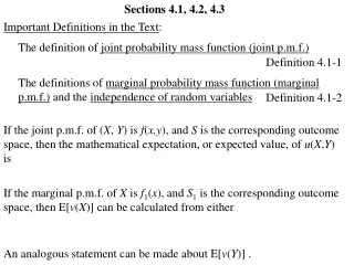
Sections 4.1, 4.2, 4.3. Important Definitions in the Text :. The definition of joint probability mass function (joint p.m.f.). Definition 4.1-1. The definitions of marginal probability mass function (marginal p.m.f.) and the independence of random variables. Definition 4.1-2.

Sections 4.1, 4.2, 4.3
E N D
Presentation Transcript
Sections 4.1, 4.2, 4.3 Important Definitions in the Text: The definition of joint probability mass function (joint p.m.f.) Definition 4.1-1 The definitions of marginal probability mass function (marginal p.m.f.) and the independence of random variables Definition 4.1-2 If the joint p.m.f. of (X, Y) is f(x,y), and S is the corresponding outcome space, then the mathematical expectation, or expected value, of u(X,Y) is If the marginal p.m.f. of X is f1(x), and S1 is the corresponding outcome space, then E[v(X)] can be calculated from either An analogous statement can be made about E[v(Y)] .
1. Twelve bags each contain two pieces of candy, one red and one green. In two of the bags each piece of candy weighs 1 gram; in three of the bags the red candy weighs 2 grams and the green candy weighs 1 gram; in three of the bags the red candy weighs 1 gram and the green candy weighs 2 grams; in the remaining four bags each piece of candy weighs 2 grams. One bag is selected at random and the following random variables are defined: X = weight of the red candy , Y = weight of the green candy . 1/4 1/3 2 y 1 1/6 1/4 The space of (X, Y) is {(1,1) (1,2) (2,1) (2,2)}. 1 2 x 1 — 6 if (x, y) = (1, 1) 1 — 4 The joint p.m.f. of (X, Y) is f(x, y) = if (x, y) = (1, 2) , (2, 1) 1 — 3 if (x, y) = (2, 2)
if x = 1 if x = 2 5 / 12 The marginal p.m.f. of X is f1(x) = 7 / 12 if y = 1 if y = 2 5 / 12 The marginal p.m.f. of Y is f2(y) = 7 / 12 A formula for the joint p.m.f. of (X,Y) is f(x, y) = x + y —— if (x, y) = (1, 1) , (1, 2) , (2, 1) , (2, 2) 12 A formula for the marginal p.m.f. of X is f1(x) = x + 1 x + 2 —— + —— = 12 12 2x + 3 ——— if x = 1, 2 12 f(x, 1) + f(x, 2) = A formula for the marginal p.m.f. of Y is f2(y) = 1 + y 2 + y —— + —— = 12 12 2y + 3 ——— if y = 1, 2 12 f(1, y) + f(2, y) =
Sections 4.1, 4.2, 4.3 Important Definitions in the Text: The definition of joint probability mass function (joint p.m.f.) Definition 4.1-1 The definitions of marginal probability mass function (marginal p.m.f.) and the independence of random variables Definition 4.1-2 If the joint p.m.f. of (X, Y) is f(x,y), and S is the corresponding outcome space, then the mathematical expectation, or expected value, of u(X,Y) is E[u(X,Y)] = u(x,y)f(x,y) (x,y) S If the marginal p.m.f. of X is f1(x), and S1 is the corresponding outcome space, then E[v(X)] can be calculated from either or v(x)f1(x) v(x)f(x,y) x S (x,y) S 1 An analogous statement can be made about E[v(Y)] .
1. - continued E(X) = (1)(5/12) + (2)(7/12) = 19/12 E(X2) = (1)2(5/12) + (2)2(7/12)= 11/4 Var(X) = 11/4 – (19/12)2= 35/144 E(Y) = (1)(5/12) + (2)(7/12) = 19/12 E(Y2) = (1)2(5/12) + (2)2(7/12)= 11/4 Var(Y) = 11/4 – (19/12)2= 35/144 Since _________________________, then the random variables X and Y _______________ independent. f(x, y) f1(x)f2(y) are not Using the joint p.m.f., E(X + Y) = (1+1)(1/6) + (1+2)(1/4) + (2+1)(1/4) + (2+2)(1/3) = 19 / 6 Alternatively, E(X + Y) = 19/12 + 19/12 = 19 / 6 E(X) + E(Y) =
Using the joint p.m.f., E(X–Y) = (1–1)(1/6) + (1–2)(1/4) + (2–1)(1/4) + (2–2)(1/3) = 0 Alternatively, E(X–Y) = 19/12 – 19/12 = 0 E(X + Y) can be interpreted as the mean of the total weight of candy in the bag. E(X–Y) can be interpreted as the mean of how much more the red candy in the bag weighs than the green candy. E(XY) = (1)(1)(1/6) + (1)(2)(1/4) + (2)(1)(1/4) + (2)(2)(1/3) = 5/2 Cov(X,Y) =
1. - continued = The least squares lines for predicting Y from X is The least squares lines for predicting X from Y is
The conditional p.m.f. of Y | X = 1 is Y | X = 2 is For x = 1, 2, a formula for the conditional p.m.f. of Y | X = x is
1. - continued The conditional p.m.f. of X | Y = 1 is X | Y = 2 is For y = 1, 2, a formula for the conditional p.m.f. of X | Y = y is
E(Y | X = 1) = E(Y2 | X = 1) = Var(Y | X = 1) = E(Y | X = 2) = E(Y2 | X = 2) = Var(Y | X = 2) = Is the conditional mean of Y given X = x a linear function of the given value, that is, can we write E(Y | X = x) = a + bx ?
1. - continued E(X | Y = 1) = E(X2 | Y = 1) = Var(X | Y = 1) = E(X | Y = 2) = E(X2 | Y = 2) = Var(X | Y = 2) = Is the conditional mean of X given Y = y a linear function of the given value, that is, can we write E(X | Y = y) = c + dy ?
2. An urn contains six chips, one $1 chip, two $2 chips, and three $3 chips. Two chips are selected at random and without replacement. The following random variables are defined: X = dollar value of the first chip selected , Y = dollar value of the second chip selected . The space of (X, Y) is {(1,2) (1,3) (2,1) (2,2) (2,3) (3,1) (3,2) (3,3)}. 1/10 1/5 1/5 3 y 2 1 1/15 1/15 1/5 1/15 1/10 1 — 5 if (x, y) = (2, 3) , (3, 2) , (3, 3) 1 2 3 x 1 — 10 if (x, y) = (1, 3) , (3, 1) The joint p.m.f. of (X, Y) is f(x, y) = 1 — 15 if (x, y) = (1, 2) , (2, 1) , (2, 2)
2. - continued if x = 1 if x = 2 if x = 3 1 / 6 The marginal p.m.f. of X is f1(x) = 1 / 3 1 / 2 if y = 1 if y = 2 if y = 3 1 / 6 The marginal p.m.f. of Y is f2(y) = 1 / 3 1 / 2 A formula for the joint p.m.f. of (X,Y) is f(x, y) = (There seems to be no easy formula.) A formula for the marginal p.m.f. of X is f1(x) = x / 6 if x = 1, 2, 3 A formula for the marginal p.m.f. of Y is f2(y) = y / 6 if y = 1, 2, 3
E(X) = 7 / 3 E(X2) = 6 Var(X) = 6 – (7 / 3)2 = 5 / 9 E(Y) = 7 / 3 E(Y2) = 6 Var(Y) = 6 – (7 / 3)2 = 5 / 9 Since _________________________, then the random variables X and Y _______________ independent. f(x, y) f1(x)f2(y) are not P(X + Y < 4) = P[(X,Y) = (1,2)] + P[(X,Y) = (2,1)] = 1 / 15 + 1 / 15 = 2 / 15 Using the joint p.m.f., E(XY) = (1)(2)(2/30) + (1)(3)(3/30) + (2)(1)(2/30) + (2)(2)(2/30) + (2)(3)(6/30) + (3)(1)(3/30) + (3)(2)(6/30) + (3)(3)(6/30) = 16 / 3
2. - continued Cov(X,Y) = = The least squares lines for predicting Y from X is The least squares lines for predicting X from Y is
The conditional p.m.f. of Y | X = 1 is Y | X = 2 is Y | X = 3 is For x = 1, 2, 3, a formula for the conditional p.m.f. of Y | X = x is
2. - continued The conditional p.m.f. of X | Y = 1 is X | Y = 2 is X | Y = 3 is For y = 1, 2, 3, a formula for the conditional p.m.f. of X | Y = y is
E(Y | X = 1) = E(X | Y = 1) = E(Y2 | X = 1) = E(X2 | Y = 1) = Var(Y | X = 1) = Var(X | Y = 1) = E(Y | X = 2) = E(X | Y = 2) = E(Y2 | X = 2) = E(X2 | Y = 2) = Var(Y | X = 2) = Var(X | Y = 2) = E(Y | X = 3) = E(X | Y = 3) = E(Y2 | X = 3) = E(X2 | Y = 3) = Var(Y | X = 3) = Var(X | Y = 3) =
2. - continued Is the conditional mean of Y given X = x a linear function of the given value, that is, can we write E(Y | X = x) = a + bx ? Is the conditional mean of X given Y = y a linear function of the given value, that is, can we write E(X | Y = y) = c + dy ?
3. An urn contains six chips, one $1 chip, two $2 chips, and three $3 chips. Two chips are selected at random and with replacement. The following random variables are defined: X = dollar value of the first chip selected , Y = dollar value of the second chip selected . The space of (X, Y) is {(1,1) (1,2) (1,3) (2,1) (2,2) (2,3) (3,1) (3,2) (3,3)}. 3 y 2 1 1/12 1/6 1/4 1/18 1/9 1/6 1/36 1/18 1/12 1 2 3 x xy — 36 x = 1, 2, 3 if y = 1, 2, 3 The joint p.m.f. of (X, Y) is f(x, y) =
3. - continued if x = 1 if x = 2 if x = 3 1 / 6 The marginal p.m.f. of X is f1(x) = 1 / 3 1 / 2 if y = 1 if y = 2 if y = 3 1 / 6 The marginal p.m.f. of Y is f2(y) = 1 / 3 1 / 2 A formula for the joint p.m.f. of (X,Y) is f(x, y) = (The formula was found previously) A formula for the marginal p.m.f. of X is f1(x) = x / 6 if x = 1, 2, 3 A formula for the marginal p.m.f. of Y is f2(y) = y / 6 if y = 1, 2, 3
E(X) = 7 / 3 E(X2) = 6 Var(X) = 6 – (7 / 3)2 = 5 / 9 E(Y) = 7 / 3 E(Y2) = 6 Var(Y) = 6 – (7 / 3)2 = 5 / 9 Since _________________________, then the random variables X and Y _______________ independent. f(x, y) =f1(x)f2(y) are P(X + Y < 4) = P[(X,Y) = (1,1)] + P[(X,Y) = (1,2)] + P[(X,Y) = (2,1)] = 1 / 36 + 1 / 18 + 1 / 18 = 5 / 36
3. - continued 3 3 (xy) (xy / 36) = x = 1 y = 1 3 3 (xy) (x / 6) (y / 6) = x = 1 y = 1 E(XY) = 3 3 (x) (x / 6) (y) (y / 6) = x = 1 y = 1 E(X) E(Y) = (7/3)(7/3) = 49 / 9 Cov(X,Y) = = The least squares lines for predicting Y from X is The least squares lines for predicting X from Y is
For x = 1, 2, 3, the conditional p.m.f. of Y | X = x is E(Y | X = x) = Var(Y | X = x) = For y = 1, 2, 3, the conditional p.m.f. of X | Y = y is E(X | Y = y) = Var(X | Y = y) = Is the conditional mean of Y given X = x a linear function of the given value, that is, can we write E(Y | X = x) = a + bx ? Is the conditional mean of X given Y = y a linear function of the given value, that is, can we write E(X | Y = y) = c + dy ?
For continuous type random variables (X, Y), the definitions of joint probability density function (joint p.d.f.), independence of X and Y, and mathematical expectation are each analogous to those for discrete type random variables, with summation signs replaced by integral signs. The covariance between random variables X and Y is The correlation between random variables X and Y is y Consider the equation of a line y = a + bx which comes “closest” to predicting the values of the random variable Y from the random variable X in the sense that E{[Y– (a + bX)]2} is minimized. x
We let k(a,b) = E{[Y – (a + bX)]2} = To minimize k(a,b) , we set the partial derivatives with respect to a and b equal to zero. (Note: This is textbook exercise 4.2-5.) k — = a k — = b (Multiply the first equation by X, subtract the resulting equation from the second equation, and solve for b. Then substitute in place of b in the first equation to solve for a.)
b = The least squares line for predicting Y from X is a = The least squares line for predicting Y from X can be written The least squares line for predicting X from Y can be written
The conditional p.m.f./p.d.f. of Y given X = x is defined to be The conditional p.m.f./p.d.f. of X given Y = y is defined to be The conditional mean of Y given X = x is defined to be The conditional variance of Y given X = x is defined to be
The conditional mean of X given Y = y and the conditional variance of X given Y = y are each defined similarly. For continuous type random variables (X, Y), the definitions of conditional mean and variance are each analogous to those for discrete type random variables, with summation signs replaced by integral signs. Suppose X and Y are two discrete type random variables, and E(Y | X = x) = a + bx. Then, for each possible value of x, Multiplying each side by f1(x), Summing each side over all x,
Now, multiplying each side of by x f1(x), Summing each side over all x,
The two equations and are essentially the same as those in the derivation of the least squares line for predicting Y from X. This derivation is analogous for continuous type random variables with summation signs replaced by integral signs. Consequently, if E(Y | X = x) = a + bx (i.e., if E(Y | X = x) is a linear function of x), then a and b must be respectively the intercept and slope in the least squares line for predicting Y from X. Similarly, if E(X | Y = y) = c + dy (i.e., if E(X | Y = y) is a linear function of y), then c and d must be respectively the intercept and slope in the least squares line for predicting X from Y.
Suppose a set contains N = N1 + N2 + N3 items, where N1 items are of one type, N2 items are of a second type, and N3 items are of a third type; n items are selected from the N items at random and without replacement. If the random variable X1 is defined to be the number of selected n items that are of the first type, the random variable X2 is defined to be the number of selected n items that are of the second type, and the random variable X3 is defined to be the number of selected n items that are of the third type, then the joint distribution of (X1 , X2 , X3) is called a trivariate hypergeometric distribution. Since X3 = n – X1 – X2 , X3 is totally determined by X1 and X2 . The joint p.m.f. of (X1 , X2) is Each Xi has a distribution. If the number of types of items is any integer k > 1 with (X1 , X2 , … , Xk) defined in the natural way, then the joint p.d.f. is called a multivariate hypergeometric distribution.
Suppose each in a sequence of independent trials must result in one of outcome 1, outcome 2, or outcome 3. The probability of outcome 1 on each trial is p1 , the probability of outcome 2 on each trial is p2 , and the probability of outcome 3 on each trial is p3 = 1 – p1 – p2 . If the random variable X1 is defined to be the number of the n trials resulting in outcome 1, the random variable X2 is defined to be the number of the n trials resulting in outcome 2, and the random variable X3 is defined to be the number of the n trials resulting in outcome 3, then the joint distribution of (X1 , X2 , X3) is called a trinomial distribution. Since X3 = n – X1 – X2 , X3 is totally determined by X1 and X2 . The joint p.m.f. of (X1 , X2) is Each Xi has a distribution. If the number of outcomes is any integer k > 1 with (X1 , X2 , … , Xk) defined in the natural way, then the joint p.d.f. is called a multinomial distribution.
4. (a) An urn contains 15 red chips, 10 blue chips, and 5 white chips. Eight chips are selected at random and without replacement. The following random variables are defined: X1 = number of red chips selected , X2 = number of blue chips selected , X3 = number of white chips selected . Find the joint p.m.f. of (X1 , X2 , X3) . (X1 , X2 , X3) have a trivariate hypergeometric distribution, and X3 = 8 –X1–X2 is totally determined by X1 and X2 . The joint p.m.f. of (X1 , X2) is 15 x1 10 x2 5 8 – x1 – x2 x1 = 0, 1, …, 8 if x2 = 0, 1, …, 8 f(x1, x2) = 30 8 3 x1 + x2 8
(b) Find the marginal p.m.f. for each of X1 , X2 , and X3 . Each of X1 , X2 , and X3 has a hypergeometric distribution. 15 x1 15 8 – x1 f1(x1) = if x1 = 0, 1, …, 8 30 8 10 x2 20 8 – x2 f2(x2) = if x2 = 0, 1, …, 8 30 8
4. - continued (c) 5 x3 25 8 – x3 f3(x3) = if x3 = 0, 1, …, 5 30 8 Are X1 , X2 , and X3 independent? Why or why not? X1, X2, X3 cannot possibly be independent, because any one of these random variables is totally determined by the other two.
(d) Find the probability that at least two of the selected chips are blue or at least two chips are white. P({X2 2} {X3 2}) = 1 – P({X2 1} {X3 1}) = 1 – [P(X2= 0 ,X3 = 0) + P(X2= 1 ,X3 = 0) + P(X2= 0 ,X3 = 1) + P(X2= 1 ,X3 = 1)] = 15 8 15 7 10 1 15 7 5 1 15 6 10 1 5 1 1 – + + + 30 8 30 8 30 8 30 8
4. - continued (e) (f) Find the conditional p.m.f. of X1 | x2 . X1 | x2 can be treated as “the number of red chips selected when For x2 = X1 | x2 has a distribution with p.m.f. E(X1 | x2) can be written as a linear function of x2 , since Therefore, the least squares E(X1 | x2) =
line for predicting X1 from X2 must be (g) E(X2 | x1) can be written as a linear function of x2 , since E(X2 | x1) = Therefore, the least squares line for predicting X2 from X1 must be (h) Find the covariance and correlation between X1 and X2 by making use of the following facts (instead of using direct formulas): The slope in the least squares line for predicting X1 from X2 is The slope in the least squares line for predicting X2 from X1 is The product of the slope in the least squares line for predicting X1 from X2 and the slope in the least squares line for predicting X2 from X1 is equal to .
Suppose a set contains N = N1 + N2 + N3 items, where N1 items are of one type, N2 items are of a second type, and N3 items are of a third type; n items are selected from the N items at random and without replacement. If the random variable X1 is defined to be the number of selected n items that are of the first type, the random variable X2 is defined to be the number of selected n items that are of the second type, and the random variable X3 is defined to be the number of selected n items that are of the third type, then the joint distribution of (X1 , X2 , X3) is called a trivariate hypergeometric distribution. Since X3 = n – X1 – X2 , X3 is totally determined by X1 and X2 . N1 x1 N2 x2 N – N1– N2 n – x1–x2 The joint p.m.f. of (X1 , X2) is if x1 and x2 are “appropriate” integers N n Each Xi has a distribution. If the number of types of items is any integer k > 1 with (X1 , X2 , … , Xk) defined in the natural way, then the joint p.d.f. is called a multivariate hypergeometric distribution. hypergeometric
5. (a) An urn contains 15 red chips, 10 blue chips, and 5 white chips. Eight chips are selected at random and with replacement. The following random variables are defined: X1 = number of red chips selected , X2 = number of blue chips selected , X3 = number of white chips selected . Find the joint p.m.f. of (X1 , X2 , X3) . (X1 , X2 , X3) have a trinomial distribution, and X3 = 8 –X1–X2 is totally determined by X1 and X2 . The joint p.m.f. of (X1 , X2) is x1 x2 8 –x1–x2 8! 1 — 2 1 — 3 1 — 6 f(x1, x2) = x1! x2! (8 –x1–x2)! x1 = 0, 1, …, 8 if x2 = 0, 1, …, 8 x1 + x2 8
(b) Find the marginal p.m.f. for each of X1 , X2 , and X3 . Each of X1 , X2 , and X3 has a binomial distribution. 8 8! 1 — 2 f1(x1) = if x1 = 0, 1, …, 8 x1! (8 –x1)! x2 8 – x2 8! 1 — 3 2 — 3 f2(x2) = if x2 = 0, 1, …, 8 x2! (8 –x2)!
5. - continued (c) x3 8 – x3 8! 1 — 6 5 — 6 f3(x3) = if x3 = 0, 1, …, 8 x3! (8 –x3)! Are X1 , X2 , and X3 independent? Why or why not? X1, X2, X3 cannot possibly be independent, because any one of these random variables is totally determined by the other two.
(d) Find the probability that at least two of the selected chips are blue or at least two chips are white. P({X2 2} {X3 2}) = 1 – P({X2 1} {X3 1}) = 1 – [P(X2= 0 ,X3 = 0) + P(X2= 1 ,X3 = 0) + P(X2= 0 ,X3 = 1) + P(X2= 1 ,X3 = 1)] = 8 7 8! 1 — 2 1 — 2 1 — 3 1 – + + 7! 1! 7 6 8! 8! 1 — 2 1 — 6 1 — 2 1 — 3 1 — 6 + 7! 1! 6! 1! 1!
5. - continued (e) (f) Find the conditional p.m.f. of X1 | x2 . X1 | x2 can be treated as “the number of red chips selected when For x2 = X1 | x2 has a distribution with p.m.f. E(X1 | x2) can be written as a linear function of x2 , since Therefore, the least squares E(X1 | x2) =
line for predicting X1 from X2 must be (g) E(X2 | x1) can be written as a linear function of x2 , since E(X2 | x1) = Therefore, the least squares line for predicting X2 from X1 must be (h) Find the covariance and correlation between X1 and X2 by making use of the following facts (instead of using direct formulas): The slope in the least squares line for predicting X1 from X2 is The slope in the least squares line for predicting X2 from X1 is The product of the slope in the least squares line for predicting X1 from X2 and the slope in the least squares line for predicting X2 from X1 is equal to .
Suppose each in a sequence of independent trials must result in one of outcome 1, outcome 2, or outcome 3. The probability of outcome 1 on each trial is p1 , the probability of outcome 2 on each trial is p2 , and the probability of outcome 3 on each trial is p3 = 1 – p1 – p2 . If the random variable X1 is defined to be the number of the n trials resulting in outcome 1, the random variable X2 is defined to be the number of the n trials resulting in outcome 2, and the random variable X3 is defined to be the number of the n trials resulting in outcome 3, then the joint distribution of (X1 , X2 , X3) is called a trinomial distribution. Since X3 = n – X1 – X2 , X3 is totally determined by X1 and X2 . The joint p.m.f. of (X1 , X2) is x1 x2 n–x1–x2 n! p1p2 (1 –p1–p2) x1! x2! (n–x1–x2)! if x1 and x2 are non-negative integers such that x1 + x2n Each Xi has a distribution. If the number of outcomes is any integer k > 1 with (X1 , X2 , … , Xk) defined in the natural way, then the joint p.d.f. is called a multinomial distribution. b( , ) n pi
6. One chip is selected from each of two urns, one containing three chips labeled distinctively with the integers 1 through 3 and the other containing two chips labeled distinctively with the integers 1 and 2. The following random variables are defined: X = largest integer among the labels on the selected chips , Y = smallest integer among the labels on the selected chips . The space of (X, Y) is {(1,1) (2,1) (3,1) (2,2) (3,2)}. 1/6 1/6 2 y 1 (Note: We immediately see that X and Y cannot be independent, since the joint space is not “rectangular”.) 1/6 1/3 1/6 1 2 3 x The joint p.m.f. of (X, Y) is f(x, y) = 1 — 6 if (x, y) = (1, 1) , (3, 1) , (2, 2) , (3, 2) 1 — 3 if (x, y) = (2, 1)
if x = 1 if x = 2, 3 1 / 6 The marginal p.m.f. of X is f1(x) = 1 / x The marginal p.m.f. of Y is f2(y) = (3 – y) / 3 if y = 1, 2 E(X) = 13 / 6 E(X2) = 31 / 6 Var(X) = 31 / 6 – (13 / 6)2 = 17 / 36 E(Y) = 4 / 3 E(Y2) = 2 Var(Y) = 2 – (4 / 3)2 = 2 / 9
6. - continued Since _________________________, then the random variables X and Y _______________ independent f(x, y) f1(x)f2(y) are not (as we previously noted). Using the joint p.m.f., E(XY) = (1)(1)(1/6) + (3)(1)(1/6) + (2)(2)(1/6) + (3)(2)(1/6) + (2)(1)(1/3) = 3 Cov(X,Y) = = The least squares lines for predicting Y from X is