Continuous observations (every 30 minutes):

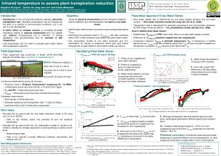
1. Infrared temperature to assess plant transpiration reduction Angelica Durigon1*, Quirijn de Jong van Lier1 and Klaas Metselaar 1Department of Biosystems Engineering, ESALQ-University of São Paulo, Brazil. *adurigon@esalq.usp.br 2Department of Environmental Sciences, Wageningen University and Research Centre, The Netherlands. EGU General Assembly, April 3-8, 2011, Vienna, Austria HS 8.3 Subsurface Hydrology - Unsaturated Zone HS 8.3.1: Soil-plant interactions from the rhizosphere to field scale University of São Paulo • Introduction • Resistances in the soil-plant-atmosphere pathway determine transpiration rate. Stomatal conductance can be changed by the plant in a reaction to environmental conditions, e.g. a dry soil or a dry atmosphere. • A direct effect of stomata closure is increased stomatal resistance leading to reduced transpiration and CO2-uptake rate. Indirect consequences are a reduction in energy dissipation and photosynthesis and an increase in leaf temperature. • Leaf temperature can be used to evaluate plant water status and transpiration reduction. • Objective • Study the physical mechanisms and the interaction between factors related to soil and atmosphere that lead to crop water stress. • Identify plant water stress occurrence using canopy temperature Tcanopy. • Determine how pressure head h, ∆Tcanopy-air and vapor pressure deficit VPD in field conditionsare related with plant water stress. • Use mechanistic models of root water extraction and CO2 assimilation by leaves to determine which part (soil and/or atmosphere) is responsible for plant water stress occurrence. Theoretical Aspects of Crop Water Stress • Root water uptake rate is determined by root water uptake dynamic and soil water content → Root water extraction model (De Jong van Lier et al., 2008) • Transpiration rate is determined by stomatal conductance and microclimatic elements, as VPD (Vapor Pressure Deficit) → CO2 Assimilation model (Jacobs et al., 1996) How to identify plant water stress? • Relationship ∆Tcanopy-air x VPD: linear when there is enough water supply to plants. • Difference of ∆Tcanopy-air between irrigated and non irrigated plot. • Comparison between Tcanopy x wet-bulb temperature Twb: if resistances in healthy plants are low, Tcanopy must be constantly higher than Twb; as soon as plant resistance to transpiration increases, Tcanopy become even higher than Twb. • Field Experiment • Field experiment was performed in Brazil (UTM 253.300E, latitude 153.400N) from June/2010 to September/2010. Identifying Plant Water Stress • ∆Tcanopy-air x VPD (02-Aug to 02-Sep) 1 - Plants of non irrigated plot were water stressed. 4 - Water stress decreased in 16-Aug as VPD reduced. 5 - Even with a high VPD difference in 25-Aug, water stress reduced as soil water content increased. 02/07/2010 19/07/2010 BEANS (Phaseolus vulgaris L.) Area: 990 m2 (22 m x 45 m) Two plots: 22 m x 22,5 m (one irrigated) Dry period: 02-Aug to 02-Sep 2 - Plants of irrigated plot were not water stressed (linear relationship). 3 - Water stress started on 5-Aug (comparing both plots and considering plants in irrigated plot were non water stressed). Fig. 1: Experimental site. Fig. 3: Difference of ∆Tcanopy-air and VPD between non irrigated (nir) and irrigated (ir) plots Continuous observations (every 30 minutes): • Pressure head h(Polymer Tensiometers measuring till -1.6 MPa): 2 observation points each plot at 0.05, 0.15 and 0.30 m depth. • Tair and RH: 1 observation point each plot. • Tcanopy: 1 observation point each plot (infrared thermometry). • ∆Tcanopy-air and VPD between plots • Pressure head h - non irrigated plot Campaign observations: • Root density: 3 times each plot. • Stomatal resistance and transpiration rate: 11 days at midday. • Leaf Area Index (LAI): 5 times with a ceptometer. Fig. 2: ∆Tcanopy-air x VPD for irrigated plot (above) and non irrigated plot (below). Next steps • Simulate the dry period with the root water extraction model of De Jong van Lier et al. (2008): • Data of root density, matric flux potential M and soil hydraulic parameters. • Simulate the dry period with the CO2 assimilation model of Jacobs et al. (1996) to identify the midday depression in photosynthesis in plants of both plots: • Meteorological data. • Data of Ds (specific humidity difference between atmosphere and leaves) and LAI. • Tcanopy and Twb Fig. 4: Pressure head h for both observation points of non irrigated plot 6 - Tcanopy is higher than Twb for both plots. 7 - ΔTcanopy-wb is approximately constant during whole period for irrigated plot but increases for non irrigated plot. 8 - At the end of the month, Tcanopy of non irrigated plot becomes even higher than Twb indicating an increment in stomatal resistance to transpiration. 9 - Although atmospheric demand was the same for both plots, hydrological parameters differed significantly between them. 10 - Pressure head dropped down to -150.0 m in non irrigated plot and at this time Tcanopy presented its maximum values (~ 38.0°C). Preliminar conclusion:Sometimes observed plant water stress was a combined effect of soil and atmosphere, on other ocassions it has been a single effect of soil or atmosphere. Fig. 5: Difference between Tcanopy and Twb for non irrigated and irrigated plots. Main Bibliographic References Bakker et al. (2007). New polymer tensiometers: measuring matric pressures down to wilting point. Vadose Z.J., 6, 196-202. De Jong van Lier et al. (2008) Macroscopic root water uptake distribution using a matric flux potential approach. Vadose Z. J., p. 1065-1078. Ehrler (1973). Cotton leaf temperatures as related to soil water depletion and meteorological factors. Agron. J., 65, 404-409. Fucks (1990). Infrared measurement of canopy temperature and detection of plant water stress. Theor. Appl. Climatol., 42, 253-261. Idso et al. (1981). Normalizing the stress-degree-day parameter for environmental variability. Agricultural Meteorology, 24, 45–55. Jacobs et al. (1996) Stomatal behavior and photosynthetic rate of unstressed grapevines in semi-arid conditions. Agricultural and Forest Meteorology, 2, 111-134. Shimoda and Oikawa (2006). Temporal and spatial variations of canopy temperature over a C3-C4 mixture grassland. Hydrol. Process., 20, 3503-3516. Tanner (1963). Plant temperature. Agron. J., 55, 210-211. Van der Ploeg et al. (2008). Matric potential measurements by polymer tensiometers in cropped lysimeters under water-stressed conditions. Vadose Z. J., 7, 1048-1054. Acknowledgements CAPES-WUR Agreement (proj. n.° 019/06) WUR/The Netherlands (proj. n.° 5100184-01) FAPESP (proj. n.° 2009/02117-7) University of São Paulo - Post-Graduation Section