
Aliasing in Image Rendering through Sampling Theory
E N D
Presentation Transcript
Sampling and Aliasing Kurt Akeley CS248 Lecture 3 2 October 2007 http://graphics.stanford.edu/courses/cs248-07/
Aliasing Aliases are low frequencies in a rendered image that are due to higher frequencies in the original image.
Jaggies Original: Rendered: Are jaggies due to aliasing? How?
What is a point sample (aka sample)? An evaluation • At an infinitesimal point (2-D) • Or along a ray (3-D) What is evaluated • Inclusion (2-D) or intersection (3-D) • Attributes such as distance and color
Why point samples? Clear and unambiguous semantics Matches theory well (as we’ll see) Supports image assembly in the framebuffer • will need to resolve visibility based on distance, and this works well with point samples Anything else just puts the problem off • Exchange one large, complex scene for many small, complex scenes
Fourier theory “Fourier’s theorem is not only one of the most beautiful results of modern analysis, but it may be said to furnish an indispensable instrument in the treatment of nearly every recondite question in modern physics.” -- Lord Kelvin
Reference sources Marc Levoy’s notes Ronald N. Bracewell, The Fourier Transform and its Applications, Second Edition, McGraw-Hill, Inc., 1978. Private conversations with Pat Hanrahan MATLAB
Ground rules You don’t have to be an engineer to get this • We’re looking to develop instinct / understanding • Not to be able to do the mathematics We’ll make minimal use of equations • No integral equations • No complex numbers Plots will be consistent • Tick marks at unit distances • Signal on left, Fourier transform on the right
Dimensions 1-D • Audio signal (time) • Generic examples (x) 2-D • Image (x and y) 3-D • Animation (x, y, and time) All examples in this presentation are 1-D
Fourier series Any periodic function can be exactly represented by a (typically infinite) sum of harmonic sine and cosine functions. Harmonics are integer multiples of the fundamental frequency
Fourier series example: sawtooth wave 1 … … -1 1
Sawtooth wave summation 1 2 3 n Harmonics Harmonic sums
Sawtooth wave summation (continued) 5 10 50 n Harmonics Harmonic sums
Fourier integral Any function (that matters in graphics) can be exactly represented by an integration of sine and cosine functions. Continuous, not harmonic But the notion of harmonics will continue to be useful
Basic Fourier transform pairs II(s) f(x) F(s)
Reciprocal property Swapped left/right from previous slide II(s) f(x) F(s)
Scaling theorem II(2s) II(s/2) f(x) F(s)
Band-limited transform pairs sinc(x) sinc2(x) f(x) F(s)
Finite / infinite extent If one member of the transform pair is finite, the other is infinite • Band-limited infinite spatial extent • Finite spatial extent infinite spectral extent
Convolution theorem Let fand g be the transforms of f and g. Then Something difficult to do in one domain (e.g., convolution) may be easy to do in the other (e.g., multiplication)
Sampling theory x * Spectrum is replicated an infinite number of times = = f(x) F(s)
Reconstruction theory * x sinc = = f(x) F(s)
Sampling at the Nyquist rate x * = = f(x) F(s)
Reconstruction at the Nyquist rate * x = = f(x) F(s)
Sampling below the Nyquist rate x * = = f(x) F(s)
Reconstruction below the Nyquist rate * x = = f(x) F(s)
Reconstruction error Original Signal UndersampledReconstruction
Reconstruction with a triangle function * x = = f(x) F(s)
Reconstruction error Original Signal TriangleReconstruction
Reconstruction with a rectangle function * x = = f(x) F(s)
Reconstruction error Original Signal RectangleReconstruction
Sampling a rectangle x * = = f(x) F(s)
Reconstructing a rectangle (jaggies) * x = = f(x) F(s)
Sampling and reconstruction Aliasing is caused by • Sampling below the Nyquist rate, • Improper reconstruction, or • Both We can distinguish between • Aliasing of fundamentals (demo) • Aliasing of harmonics (jaggies)
Summary Jaggies matter • Create false cues • Violate rule 1 Sampling is done at points (2-D) or along rays (3-D) • Sufficient for depth sorting • Matches theory Fourier theory explains jaggies as aliasing. For correct reconstruction: • Signal must be band-limited • Sampling must be at or above Nyquist rate • Reconstruction must be done with a sinc function
Assignments Before Thursday’s class, read • FvD 3.17 Antialiasing Project 1: • Breakout: a simple interactive game • Demos Wednesday 10 October