Download

1 / 39
390 likes | 565 Vues
Data Warehouse implementation: Part B. Dr . Panagiotis S ymeonidis Data Engineering Laboratory. http://delab.csd.auth.gr/~symeon. Cuboids Materialization as an Optimization Problem. Minimize : the average time taken to evaluate a view Constraint : materialize a fixed number k of views

E N D
Data Warehouse implementation: PartB Dr. Panagiotis Symeonidis Data Engineering Laboratory http://delab.csd.auth.gr/~symeon
Cuboids Materialization as an Optimization Problem • Minimize: the average time taken to evaluate a view • Constraint: materialize a fixed number k of views Greedy algorithm • Best choice is given based on what has gone before • It does not give the optimal solution
Example of lattice of views diagram psc p: parts: suppc: cust pc ps sc p s c
The lattice of views framework • if view V2 can be answered using results of view V1 then • V2 is descendent of V1 • V1 is ancestor of V2 • (denoted V2 ≼ V1) • E.g. (part) ≼ (part, cust)
Some Definitions • K is the number of views to be materialized • C (v ) is the cost of view v • Given • v is a view • S is a set of views which are already selected to be materialized • The Benefit of selecting v for materialization is • B(v, S) = C(S) – C(S U v)
Greedy Algorithm • S {top view}; • For i = 1 to k do • Select that view v not in S such that B(v, S) is maximized; • S S U {v} • Return S
Benefit from pc = pc 6M ps 0.8M sc 6M p 0.2M s 0.01M c 0.1M 6M-6M = 0 1.1 Data Cube psc 6M k = 2 Benefit = 0 0 x 3
Benefit from ps = pc 6M ps 0.8M sc 6M p 0.2M s 0.01M c 0.1M 6M-0.8M = 5.2M 1.1 Data Cube psc 6M k = 2 Benefit = 0 0 x 3 = 15.6 5.2 x 3
Benefit from sc = pc 6M ps 0.8M sc 6M p 0.2M s 0.01M c 0.1M 6M-6M = 0 1.1 Data Cube psc 6M k = 2 Benefit = 0 0 x 3 = 15.6 5.2 x 3 = 0 0 x 3
Benefit from p = pc 6M ps 0.8M sc 6M p 0.2M s 0.01M c 0.1M 6M-0.2M = 5.8M 1.1 Data Cube psc 6M k = 2 Benefit = 0 0 x 3 = 15.6 5.2 x 3 = 0 0 x 3 = 5.8 5.8 x 1
Benefit from s = pc 6M ps 0.8M sc 6M p 0.2M s 0.01M c 0.1M 6M-0.01M = 5.99M 1.1 Data Cube psc 6M k = 2 Benefit = 0 0 x 3 = 15.6 5.2 x 3 = 0 0 x 3 = 5.8 5.8 x 1 = 5.99 5.99 x 1
Benefit from c = pc 6M ps 0.8M sc 6M p 0.2M s 0.01M c 0.1M 6M-0.1M = 5.9M 1.1 Data Cube psc 6M k = 2 Benefit = 0 0 x 3 = 15.6 5.2 x 3 = 0 0 x 3 = 5.8 5.8 x 1 = 5.99 5.99 x 1 = 5.9 5.9 x 1
Benefit from pc = pc 6M ps 0.8M sc 6M p 0.2M s 0.01M c 0.1M 6M-6M = 0 1.1 Data Cube psc 6M k = 2 Benefit = 0 0 x 3 = 0 0 x 2 = 15.6 5.2 x 3 = 0 0 x 3 = 5.8 5.8 x 1 = 5.99 5.99 x 1 = 5.9 5.9 x 1
Benefit from sc = pc 6M ps 0.8M sc 6M p 0.2M s 0.01M c 0.1M 6M-6M = 0 1.1 Data Cube psc 6M k = 2 Benefit = 0 0 x 3 = 0 0 x 2 = 15.6 5.2 x 3 = 0 = 0 0 x 3 0 x 2 = 5.8 5.8 x 1 = 5.99 5.99 x 1 = 5.9 5.9 x 1
pc 6M ps 0.8M sc 6M p 0.2M s 0.01M c 0.1M psc 6M k = 2 Benefit from p = 0.8M-0.2M = 0.6M Benefit = 0 0 x 3 = 0 0 x 2 = 15.6 5.2 x 3 = 0 = 0 0 x 3 0 x 2 = 5.8 = 0.6 5.8 x 1 0.6 x 1 = 5.99 5.99 x 1 = 5.9 5.9 x 1
pc 6M ps 0.8M sc 6M p 0.2M s 0.01M c 0.1M 1.1 Data Cube psc 6M k = 2 Benefit from s = 0.8M-0.01M = 0.79M Benefit = 0 0 x 3 = 0 0 x 2 = 15.6 5.2 x 3 = 0 = 0 0 x 3 0 x 2 = 5.8 = 0.6 5.8 x 1 0.6 x 1 = 5.99 = 0.79 5.99 x 1 0.79 x 1 = 5.9 5.9 x 1
pc 6M ps 0.8M sc 6M p 0.2M s 0.01M c 0.1M 1.1 Data Cube psc 6M Benefit from c = k = 2 6M-0.1M = 5.9M Benefit = 0 0 x 3 = 0 0 x 2 = 15.6 5.2 x 3 = 0 = 0 0 x 3 0 x 2 = 5.8 = 0.6 5.8 x 1 0.6 x 1 = 5.99 = 0.79 5.99 x 1 0.79 x 1 = 5.9 5.9 x 1 = 5.9 5.9 x 1
pc 6M ps 0.8M sc 6M p 0.2M s 0.01M c 0.1M psc 6M k = 2 Benefit • Two views to be materialized are • ps • c = 0 0 x 3 = 0 0 x 2 = 15.6 5.2 x 3 = 0 = 0 0 x 3 0 x 2 = 5.8 = 0.6 5.8 x 1 0.6 x 1 = 5.99 = 0.79 V = {ps, c} Gain(V U {top view}, {top view}) = 15.6 + 5.9 = 21.5 5.99 x 1 0.79 x 1 = 5.9 5.9 x 1 = 5.9 5.9 x 1
100 a 75 50 b c d e f 20 30 40 g h 1 10 2nd Example of greedy algorithm • Initially, S = {a} • k = 4 (select 3 more)
2nd Example of greedy algorithm 100 First choice • b: 50 5 = 250 • c: 25 5 = 125 • d: 80 2 = 160 • e: 70 3 = 210 • f: 60 2 = 120 • g: 99 1 = 99 • h: 90 1 = 90 a 75 50 b c 20 30 40 d e f g h 1 10
2nd Example of greedy algorithm 100 Second choice • c: 25 2 = 50 • d: 30 2 = 60 • e: 20 3 = 60 • f: (100-40) 1 + (50-40) 1= 60+10 = 70 • g: 49 1 = 49 • h: 40 1 = 40 a 75 50 b c 20 30 40 d e f g h 1 10
2nd Example of greedy algorithm 100 Third choice • c: 25 1 = 25 • d: 30 2 = 60 • e: (50-30) 2 + (40-30) 1=20 2 + 10 1 = 50 • g: 49 1 = 49 • h: 30 1 = 30 a 75 50 b c 20 30 40 d e f g h 1 10
2nd Example of greedy algorithm 100 • If we materialize only a then cost would be 8*100 =800 • Now, cost is 800-250-70-60 = 420 a 75 50 b c 20 30 40 d e f g h 1 10
Performance Study • How bad does the Greedy Algorithm perform?
b 100 c 99 d 100 k = 2 Benefit from b = 1.1 Data Cube a 200 200-100 = 100 p1 97 q1 97 r1 97 s1 97 20 nodes … … … … p20 97 q20 97 r20 97 s20 97 Benefit = 4100 41 x 100
b 100 c 99 d 100 k = 2 Benefit from c = 1.1 Data Cube a 200 200-99 = 101 p1 97 q1 97 r1 97 s1 97 20 nodes … … … … p20 97 q20 97 r20 97 s20 97 Benefit = 4100 41 x 100 = 4141 41 x 101
b 100 c 99 d 100 k = 2 1.1 Data Cube a 200 p1 97 q1 97 r1 97 s1 97 20 nodes … … … … p20 97 q20 97 r20 97 s20 97 Benefit = 4100 41 x 100 = 4141 41 x 101 = 4100 41 x 100
b 100 c 99 d 100 k = 2 Benefit from b = 1.1 Data Cube a 200 200-100 = 100 p1 97 q1 97 r1 97 s1 97 20 nodes … … … … p20 97 q20 97 r20 97 s20 97 Benefit = 4100 41 x 100 = 2100 21 x 100 = 4141 41 x 101 = 4100 41 x 100
b 100 c 99 d 100 k = 2 1.1 Data Cube a 200 p1 97 q1 97 r1 97 s1 97 20 nodes … … … … p20 97 q20 97 r20 97 s20 97 Greedy: V = {b, c} Gain(V U {top view}, {top view}) = 4141 + 2100 = 6241 Benefit = 4100 41 x 100 = 2100 21 x 100 = 4141 41 x 101 = 2100 21 x 100 = 4100 41 x 100
b 100 c 99 d 100 = 2141 21 x 101 + 20 x 1 = 4100 41 x 100 k = 2 1.1 Data Cube a 200 p1 97 q1 97 r1 97 s1 97 20 nodes … … … … p20 97 q20 97 r20 97 s20 97 Greedy: V = {b, c} Gain(V U {top view}, {top view}) = 4141 + 2100 = 6241 Benefit = 4100 41 x 100 = 4141 41 x 101 = 4100 41 x 100 Optimal: V = {b, d} Gain(V U {top view}, {top view}) = 4100 + 4100 = 8200
b 100 c 99 d 100 Greedy Optimal 6241 = = 0.7611 8200 k = 2 1.1 Data Cube a 200 p1 97 q1 97 r1 97 s1 97 20 nodes If this ratio = 1, Greedy can give an optimal solution. If this ratio 0, Greedy may give a “bad” solution. … … … … p20 97 q20 97 r20 97 s20 97 Greedy: V = {b, c} Gain(V U {top view}, {top view}) = 4141 + 2100 = 6241 Does this ratio has a “lower” bound? Optimal: V = {b, d} Gain(V U {top view}, {top view}) = 4100 + 4100 = 8200 It is proved that this ratio is at least 0.63.
Indexing OLAP Data: Bitmap Index Relation table Index on Region Index on Type
Determining which materialized cuboid(s) should be selected for OLAP operations • Query : Find the total sales group by {product-category, province} with the condition “year = 2004”. • Which one of the 4 following materialized cuboids should be selected to process the query? 1) {year, product, city} 2) {year, product-category, country} 3) {year, product-category, province} 4) {product, province} where year = 2004
Let the query to be processed be on {product_category, province} with the condition “year = 2004”, and there are 4 materialized cuboids available: Solution: 1) {year, product, city} – it can be used. However, it costs most because product and city are of lower level 2) {year, product-category, country} – itcannot be used because country is a more general concept than province 3) {year, product_category, province} - it can be used. It could cost less than Solution 4, if there were no many year values and there are many products for each product-category. 4) {product, province} where year = 2004 - it can be used.
Iceberg queries Assume we want to find pairs of customers and items such that the customer has purchased the item at least 5 times select P.custid, P. item, sum(P.qty) from Purchases P group by P.custid, P.item having sum (P.qty) > 5 Execution plan for the query? The number of groups is very large but the answer to the query (the top of the iceberg) is usually very small
Iceberg queries select P.custid, P. item, sum(P.qty) from Purchases P group by P.custid, P.item having sum (P.qty) > 5 select P.custid from Purchases P group by P.custid having sum (P.qty) > 5 select P.item from Purchases P group by P.item having sum (P.qty) > 5 Q1 Q2 Generate (custid, item) pairs only forcustid from Q1 and item from Q2
From On-Line Analytical Processing (OLAP) to On Line Analytical Mining (OLAM) • Why online analytical mining? • High quality of data in data warehouses • OLAP-based exploratory data analysis • Easy selection of data mining functions
An OLAM System Architecture Mining query Mining result Layer4 User Interface User GUI API OLAM Engine OLAP Engine Layer3 OLAP/OLAM Data Cube API Layer2 MDDB MDDB Meta Data Database API Filtering&Integration Filtering Layer1 Data Repository Data cleaning Data Warehouse Databases Data integration
Data Warehouse implementation: PartB Dr. Panagiotis Symeonidis Data Engineering Laboratory http://delab.csd.auth.gr/~symeon