Tilt boundary
b. Tilt boundary. D. Read-Shockley model. Start with a symmetric tilt boundary composed of a wall of infinitely straight, parallel edge dislocations (e.g. based on a 100, 111 or 110 rotation axis with the planes symmetrically disposed).

Tilt boundary
E N D
Presentation Transcript
b Tilt boundary D
Read-Shockley model • Start with a symmetric tilt boundary composed of a wall of infinitely straight, parallel edge dislocations (e.g. based on a 100, 111 or 110 rotation axis with the planes symmetrically disposed). • Dislocation density (L-1) given by:1/D = 2sin(q/2)/b q/b for small angles.
Read-Shockley model • Start with a symmetric tilt boundary composed of a wall of infinitely straight, parallel edge dislocations (e.g. based on a 100, 111 or 110 rotation axis with the planes symmetrically disposed). • Dislocation density (L-1) given by:1/D = 2sin(q/2)/b q/b for small angles.
Read-Shockley contd. • For an infinite array of edge dislocations the long-range stress field depends on the spacing. Therefore given the dislocation density and the core energy of the dislocations, the energy of the wall (boundary) is estimated (r0 sets the core energy of the dislocation): • ggb = E0 q(A0 - lnq), whereE0 = µb/4π(1-n); A0 = 1 + ln(b/2πr0)
Edge dislocations interaction edges dislocations with identical b attractive repulsive X=Y Stable at X=0 for identical b; Stable at X=Y for opposite b.
1.1 LAGB experimental results • Experimental results on copper. [Gjostein & Rhines, Acta metall. 7, 319 (1959)]
1.2 Exptl. Observations <100>Tilts Twin <110>Tilts Hasson, G. C. and C. Goux (1971). “Interfacial energies of tilt boundaries in aluminum. Experimental and theoretical determination.” Scripta metallurgica5: 889-894
Rotation to Coincidence • Red and Green lattices coincide Points to be brought into coincidence
S5 relationship Red and Green lattices coincide after rotation of 2 tan-1 (1/3) = 36.9°
Rotation to achieve coincidence [Bollmann, W. (1970). Crystal Defects and Crystalline Interfaces. New York, Springer Verlag.] • Rotate lattice 1 until a lattice point in lattice 1 coincides with a lattice point in lattice 2. • Clear that a higher density of points observed for low index axis.
Aubry Transition and Strain Localization There is an interesting, subtle and quite important issue to consider here, strain localization. Suppose we do the following thought experiment: a) Take a single crystal and cut it on some plane b) Separate the two halfs c) Rotate one w.r.t. the other (we can do this with tilt boundaries as well, it is easier for a twist boundary) d) Bring them together, slowly. Obviously we have created a twist grain boundary. Are there dislocations? When the two are well separated no (except geometrically), there is no need. When the two parts are very close together there will be. Somewhere the dislocations have to appear – why? The reason is strain localization, and one can explain it this way.
Strain Localization For dislocations we have a constrant strain energy per unit length ED. All the strain is taken up by the dislocations, there is nothing else. As we bring the two parts together, the “bonding” will increase. This will create long-range elastic strains in both parts. Intuitively the strains are going to scale as the magnitude of this bonding (in some general fashion). For simplicity, let us suppose that it scales as EStrain = 1/d2 Where d is the distance between them. There is going to be a transition, with strain preferred for large d, dislocations for small d. When this occurs is called the Aubry transition (paper will be in the additional reading).
Rotation to Coincidence • Red and Green lattices coincide Points to be brought into coincidence
S5 relationship Red and Green lattices coincide after rotation of 2 tan-1 (1/3) = 36.9°
Rotation to achieve coincidence [Bollmann, W. (1970). Crystal Defects and Crystalline Interfaces. New York, Springer Verlag.] • Rotate lattice 1 until a lattice point in lattice 1 coincides with a lattice point in lattice 2. • Clear that a higher density of points observed for low index axis.