Lecture 17 Solving the Diffusion equation

1. Lecture 17Solving the Diffusion equation • Only 5 lectures left • Come to see me before the end of term • I’ve put more sample questions and answers in Phils Problems • Past exam papers • Complete solution from last lecture • Have a look at homework 2 (due in on 12/12/08) Remember Phils Problems and your notes = everything http://www.hep.shef.ac.uk/Phil/PHY226.htm

2. Introduction to PDEs In many physical situations we encounter quantities which depend on two or more variables, for example the displacement of a string varies with space and time: y(x, t). Handing such functions mathematically involves partial differentiation and partial differential equations (PDEs). Wave equation Elastic waves, sound waves, electromagnetic waves, etc. Schrödinger’s equation Quantum mechanics Diffusion equation Heat flow, chemical diffusion, etc. Laplace’s equation Electromagnetism, gravitation, hydrodynamics, heat flow. Poisson’s equation As (4) in regions containing mass, charge, sources of heat, etc.

3. The Diffusion equation In classical physics, almost all time dependent phenomena may be described by the wave equation or the diffusion equation. Smaller than the micrometer scale, diffusion is often the dominant phenomenon. The 1D diffusion equation has the form f(x, t) is the quantity that diffuses. It usually describes a chemical or heat diffusing through a region where h2 is the diffusion constant typically 1×10-4m 2s -1 for metals.

4. Introduction to PDEs Unstable equilibrium Step 1: Let the trial solution be So and Step 2: The auxiliary is then and so roots are Step 3: General solution for real roots is Step 4: Boundary conditions could then be applied to find A and B Thing to notice is that x(t) only tends towards x=0 in one direction of t, increasing exponentially in the other

5. Introduction to PDEs Harmonic oscillator Step 1: Let the trial solution be So and Step 2: The auxiliary is then and so roots are Step 3: General solution for complex is where a= 0 and b= w so Step 4: Boundary conditions could then be applied to find C and D Thing to notice is that x(t) passes through the equilibrium position (x=0) more than once !!!!

6. SUMMARY of the procedure used to solve PDEs 1. We have an equation with supplied boundary conditions 2. We look for a solution of the form 3. We find that the variables ‘separate’ 4. We use the boundary conditions to deduce the polarity of N. e.g. 5. We use the boundary conditions further to find allowed values of k and hence X(x). so 6. We find the corresponding solution of the equation for T(t). 7. We hence write down the special solutions. • By the principle of superposition, the general solution is the sum of all special • solutions.. www.falstad.com/mathphysics.html 9. The Fourier series can be used to find the particular solution at all times.

7. Before we do anything let’s think about hot stuff Consider a metal bar heated along it’s length. The ends are placed in ice water and so are held at 0ºC and the middle section is heated by a gas burner. After a while we reach an equilibrium or steady state temperature distribution along the rod which, let’s say is given by f(x), the temperature distribution plot below. x = 0 x = L for Is there a way of describing the shape of the temperature distribution in terms of an infinite series of sine terms ??????? for Yes, it’s called the Half range sine series !!!!

8. Before we do anything let’s think about hot stuff for for Half-range sine series: where So . Full solution is given in the notes, but we don’t want to waste time doing number crunching so let’s go straight to the answer…. Find So since then This describes the temperature distribution f(x) along the bar in equilibrium

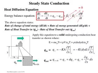
9. Solving the diffusion equation for relaxation Consider a metal bar heated along it’s length. The ends are placed in ice water and so are held at 0ºC and the middle section is heated by a gas burner. After a while we reach an equilibrium or steady state temperature distribution along the rod which, let’s say is given by f(x), the temperature distribution plot below. At t = 0 we switch off the burner and allow the rod to cool. What is the function f(x,t) that describes the temperature of the rod at any point along its length at any time as it cools? Heat flow is governed by the diffusion equation, (f is the temperature and x is position and t is time)

10. Solving the diffusion equation for relaxation Heat flow is governed by the diffusion equation, (f is the temperature and x is position and t is time) We are looking for solutions of the form Where X(x) is temperature purely as a function of x and T(t) is temperature purely as a function of time Step 1: Rewrite using new variables Substitute f(x,t) back into the Diffusion equation: Step 2: Rearrange the equation Separating variables:

11. Solving the diffusion equation for relaxation Step 3: Equate to a constant Now we have separated the variables. The above equation can only be true for all x, t if both sides are equal to a constant. which rearranges to (i) So which rearranges to (ii)

12. Solving the diffusion equation for relaxation (i) (ii) Step 4: Decide based on the boundary conditions whether constant is +ve or -ve We are told in the boundary conditions that both ends of the rod are held at 0°C at all times. We therefore choose a negative constant, –k2, to give LHO type solutions that will allow X(x) to be zero at more than one value of x, and rearrange to get two ODEs: which has general solution (iii) which has general solution (iv)

13. Solving the diffusion equation for relaxation (iii) (iv) Step 5: Solve for the boundary conditions for X(x) We know that X(0) = X(L) = 0 meaning that the temperature is zero at the ends Solution to (iii) is We know that X(0) = 0 so A = 0. so we can say Also since then X(x) x

14. Solving the diffusion equation for relaxation Step 6: Write down the special solution for fn (x, t) i.e. where So where Pn = BnCn is a special solution of the diffusion equation at one value of n

15. Solving the diffusion equation for relaxation So is a special solution of the diffusion equation at one value of n Step 7: Constructing the general solution for . The general solution of our equation is the sum of all special solutions: The general solution therefore is

16. Solving the diffusion equation for relaxation The general solution is Step 8: Use Fourier series to find values of Pn The general solution is the solution to the diffusion equation for all values of n summed from 1 to infinity. For our specific example we only want our solution to contain those harmonics required to fulfil the boundary conditions. All that remains is calculate the required values of Pn and the harmonics required. We can do this by relating the Fourier series found at t = 0 to the general solution. Remember earlier we showed that in equilibrium the temperature profile along the rod is given by: By comparing this with the general solution at the top of the page when t = 0 we can assign values to Pn .

17. Solving the diffusion equation for relaxation The general solution is Step 8 continued: Use Fourier series to find values of Pn Fourier series at t = 0 is The general solution at t = 0 is By comparing we can see that Step 9: Write down full solution of problem where

18. Solving the diffusion equation for relaxation A metal bar is heated along it’s length. The ends are placed in ice water and so are held at 0ºC and the middle section is heated by a gas burner. At t=0 heating stops. Let’s check that this fulfils all boundary conditions This is just the Fourier series at start

19. Solving the diffusion equation for relaxation A metal bar is heated along it’s length. The ends are placed in ice water and so are held at 0ºC and the middle section is heated by a gas burner. At t=0 heating stops. where Now we can stick in appropriate values of h and find how the temperature profile changes over time. It can be shown that f(x, t) with increasing time looks like this:

20. Solving the diffusion equation for relaxation Remember how we said earlier that temperature as a function of time was written: where The time constant of temperature decay is defined as , the time for temperature to drop to of its initial value. Points of interest The temperature distribution decays exponentially with time. The time constant of the decay is proportional to k -2, and therefore also L2. So the longest wavelengths (such as the fundamental) last longest. To know exactly how the temperature profile changes with time then we need all the terms. But usually a very good approximation can be obtained by considering just the first term.

21. Our experiment A good approximation can be obtained by considering just the first term. At a fixed x, the temperature drop from t = 0 is: We know p , L = 0.5m , and h2 = 3×10-5m2s-1 for stainless steel. So and therefore So We must record temperature at a fixed location on the rod at regular intervals, then plotting it as a function of time and fitting an exponential to find the decay time constant Remember that now in the full equation x is fixed constant

22. Our experiment We recorded temperature at a fixed location on the rod at regular intervals, then plotted it as a function of time and fitted an exponential to find the decay time constant Theory tells us that at a fixed x, the temperature drop from t = 0 should be: since Data collected during the lecture has a decay constant of 1.2x10-3 as expected!!!!

23. Revision for the exam http://www.shef.ac.uk/physics/exampapers/2007-08/phy226-07-08.pdf Above is a sample exam paper for this course There are 5 questions. You have to answer Q1 but then choose any 2 others Previous years maths question papers are up on Phils Problems very soon Q1: Basic questions to test elementary concepts. Looking at previous years you can expect complex number manipulation, integration, solving ODEs, applying boundary conditions, plotting functions, showing ‘x’ is solution of PDE. Easy stuff. Q2-5: More detailed questions usually centred about specific topics: InhomoODE, damped SHM equation, Fourier series, Half range Fourier series, Fourier transforms, convolution, partial differential equation solving (including applying an initial condition to general solution for a specific case), Cartesian 3D systems, Spherical polar 3D systems, Spherical harmonics The notes are the source of examinable material – NOT the lecture presentations I wont be asking specific questions about Quantum mechanics outside of the notes

24. Revision for the exam The notes are the source of examinable material – NOT the lecture presentations Things to do now Read through the notes using the lecture presentations to help where required. At the end of each section in the notes try Phils problem questions, then try the tutorial questions, then look at your problem and homework questions. If you can do these questions (they’re fun) then you’re in excellent shape for getting over 80% in the exam. Look at the past exam papers for the style of questions and the depth to which you need to know stuff. You’ll have the standard maths formulae and physical constants sheets (I’ll put a copy of it up on Phils Problems so you are sure what’s on it). You don’t need to know any equations e.g. Fourier series or transforms, wave equation, polars. Any problems – see me in my office or email me Same applies over holidays. I’ll be in the department most days but email a question or tell me you want to meet up and I’ll make sure I’m in.

25. Concerned about what you need to know? Look through previous exam questions. 2008/2009 exam will be of very similar style. You don’t need to remember any proofs or solutions (e.g. Parseval, Fourier series, Complex Fourier series) apart from damped SHM which you should be able to do. You don’t need to remember any equations or trial solutions, eg. Fourier and InhomoODE particular solutions. You don’t need to remember solutions to any PDE or for example the Fourier transform of a Gaussian and its key widths, etc. However you should understand how to solve any PDE from start to finish and how to generate a Fourier transform. Things you need to be able to do: Everything with complex numbers; solve ODEs and InhomoODEs, apply boundary conditions; integrate and differentiate general stuff; know even and odd functions; understand damped SHM, how to derive its solutions depending on damping coefficient and how to draw them; how to represent an infinitely repeating pattern as a Fourier series, how to represent a pulse as a sine or cosine half range Fourier series; how to calculate a Fourier transform; how to (de)convolve two functions; the steps needed to solve any PDE and apply boundary conditions and initial conditions (usually using Fourier series); how to integrate and manipulate equations in 3D cartesian coordinates; how to do the same in spherical polar coordinates; how to prove an expression is a solution of a spherical polar equation; explain in general terms what spherical harmonics are.