CCSM Ocean Model (POP) :
270 likes | 394 Vues
This document explores the complexities of ocean modeling using the Parallel Ocean Program (POP). It addresses the key ocean modeling problem, detailing the primitive equations governing fluid dynamics, the necessary spatial discretization through grid systems, and the algorithms to compute ocean flows. The document also discusses essential parameterizations for mixing processes, coupling techniques, and temporal discretization. Moreover, it delves into the challenges presented by irregular domains and varying spatial scales, underscoring the equilibrium time scale concerning climate modeling and energy distributions.

CCSM Ocean Model (POP) :
E N D
Presentation Transcript
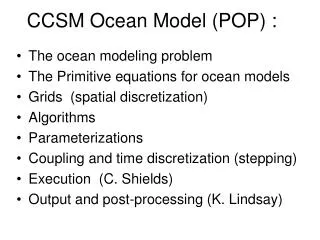
CCSM Ocean Model (POP) : • The ocean modeling problem • The Primitive equations for ocean models • Grids (spatial discretization) • Algorithms • Parameterizations • Coupling and time discretization (stepping) • Execution (C. Shields) • Output and post-processing (K. Lindsay)
The Ocean Modeling Problem • Irregular Domain - Complex coastlines - Multiply connected - Narrow straits and passages • Spatial Scales of the Flow - Eddy length scale O(10 km) - Eddy kinetic energy >> mean kinetic energy - Top, bottom and side boundary layers
The Ocean Modeling Problem • Long Equilibration Time Scale - deep adjustment time : H2/ = (5000m)2 / (10-5 m2/s) = 10,000 years • Bottom Line for Climate - Equilibrium at eddy resolution can’t be reached - Must parameterize most energetic flow
The Primative Equations • 7 equations in 7 unknowns : {U,V,W} , 3 velocity components , potential temperature S, salinity , density p, pressure • Plus 1 equation for each passive tracer, e.g. CFC, Ideal Age • Plus 1 equation for each prognostic, or diagnostic biogeochemical quantity
The Primative Equations • (1,2) Horizontal Momentum : DtU = - f k x U , Coriolis - (p/o) , pressure gradient + D(U) , lateral viscosity + ∂z(∂zU), vertical mixing - U •U , horizontal advection - w ∂zU , vertical advection
The Primative Equations • (3) Vertical Momentum : Dt W= 0 = ∂z p + g , hydrostatic • (4) Continuity : •U + ∂z W = 0 • (5) State : = (, S, p)
(5) Equation of State o = (, S, p=SLP) - 1000kg/m3 * Cabbelling : Mixing of 2 water parcels of equal density yields mixed parcel of higher density
The Primative Equations • (6) Heat : ∂t = -∂x(U ) -∂y(V ) -∂z(W ), Advection + R(, ) , Eddy mixing + ∂z (∂z - ) , Vertical mixing + ∂z SW , Solar radiation • (7) Salt : ∂t = -∂x(US) -∂y(VS) -∂z(WS) , Advection + R(, S) , Eddy mixing + ∂z (∂z S - S) , Vertical mixing
B-grid, velocity (U) and tracer (T) grids N Top View Grid Cells T T T T T T U U U U T T T T T U Land T T Land U i,j T T T T T E
B-grid, velocity (U) and tracer (T) grids z Side View Grid Cells kmt-1 T U T U T U T U T U T w w w w w kmt T U T U T U T U T w w T U T Land w w T U T KMTmax = number of levels = 40 or 25
Algorithms : Barotropic + Baroclinic Flow • Issue : CFL stability condition associated with fast (200 m/s) surface gravity waves. • Split flow into depth average barotropic plus vertically varying baroclinic • New unknowns sea surface height <U> depth averaged flow
Algorithms : 1stBaroclinic U’ • Solve for scalars ∂t(, S, T) = RHS using time delayed<U> and U’ • Explicit time marching problem (implicit vertical mixing), ∂tU’ = RHS • Surface pressure not involved
Algorithms : 2ndBarotropic <U> • Free surface boundary condition Wo = ∂t • Implicitly solve shallow water equations for ∂t + •(<U>H) = 0 Dt(H <U>) + f H (k x<U>) = g H + F(tn,n-1)
Algorithms : Advection • Conservative Flux Form X = {U,V,,S,T} : >> U • X = ∂x (UX )+ ∂y (VX) + ∂z (WX) Sum of other terms, X (•U + ∂zX) = 0 • X = ∑ An cos (n + n) discretization ==>> dispersion errors leading to “false extrema” error • Breaks 2nd law of thermodynamics : heat flows from hotter to colder.
Alternative Tracer Advection Scheme for POP • Why? Reduce dispersion errors, evidenced by artificial extrema, while not creating excessive diffusive errors • Current practice : • 3º : 2nd order centered (as for all momentum) • 1º : Upwind biased quadratic interpolation to cell faces (QUICK) • Each coordinate direction treated concurrently
CENT2 MIN north of 30°N UPWIND3 surface 0ºC 1000 -2ºC -4ºC 5000m Lax-Wendroff lim DST3 lim surface 0ºC 1000 -2ºC -4ºC 5000m
Parameterizations : KPP Vertical Mixing <wx> = ∂z Kx(∂z X -x) : X ={ U, , S, T} Diagnose boundary later depth, h, where Rib = Ric = 0.3 Ric (h) = [b(0) - b(z) + 0] h [ |U(0)-U(z)|2 + Vt2] Vt2 h wT N : <wb>e = -0.2 <wb>o ; u* 0 z <wb> he h
Parameterizations : KPP Vertical Mixing <wx> = ∂z Kx(∂z X -x) : X ={ U, , S, T} Interior -z > h, x= 0, Kx = xW + xS + xD + xC + … + …. Internal Waves : TW =10-5 m2/s**, MW = 10-4 m2/s Shear xS = f1(Rig) ; Rig = b z / |V|2 =N2 / Sh2 Double Diffusion TD = f2(R) ; R = ( ) / ( S) Convection xC =f3(Rig)
KPP Vertical Mixing <wx> = ∂z Kx(∂z X -x) : X ={ U, , S, T} Boundary Layer -z < h 0 < = -z/h < 1; Kx = h wx G() wx = u*/(u*,Bo) w* = (Bs/h)1/3as u* 0 G() = (1 + a2 + a32 ) , : Kx and its first derivative match interior at = 1 M = 0 ; T = C <wT>0 / (wx h)
Parameterizations : Eddy transport Gent McWilliams (1990) : Mimics effects of (unresolved) baroclinic eddies as a sum of (1) Diffusive mixing of scalars, R, parallel to density surfaces PLUS an additional advection of scalars by a “bolus” or eddy induced velocity , {U*, W*} : Dt X =∂t X + (U+U*) •X + (W + W*) ∂z X >>> Flattens isopycnals, thereby reducing PE >>> Dominates ACC transport (Drake Passage) and MOC (cancels much of Eulerian Deacon Cell) >>> Eliminates need for horizontal diffusion (Veronis Effect)
Parameterizations : Lateral viscosity Reynolds Stress ij = -<ui’ uj’> = (-1/3) ij <uk’uk’> + dij Deviatoric Component dij = Tijkl ekl Shear of resolved flow ekl = 0.5 [ kUl + lUk ] Tijkl a 4th order tensor with 21 of 81 elements independent T1111 = T2222 = A + B ; T3333 = A + KM ; T1212 = B T1313 = T2323 = KM ; T1133 = T2233 = B - KM Other elements 0, where not related by the symmetries Tijkl = Tjikl = Tijlk = Tklij .
Lateral viscosity Spatially Uniform, Cartesian (for illustration) D(U) = A Uxx + B UYY D(V) = B Vxx + A VYY Anisotropic A≠B, and spatially varying : satisfy numerics ONLY where needed Grid Reynolds Number Large (AUXX) or (A VYY) if required by resolution Munk: Resolve WBC Large (B VXX) only near western boundaries Strong EUC Small (B UYY )
Coupling and Time Stepping Consider a 1 day Coupling Interval with other components All daily averaged surface fluxes received, from atmosphere and sea-ice via coupler Distribute Solar Radiation 6am Noon 6pm SST, surface current Sea-ice to coupler
Coupling and Time Stepping Consider a 1 day Coupling Interval with other components All daily averaged surface fluxes received, from atmosphere and sea-ice via coupler SST, surface current Sea-ice to coupler Distribute Solar Radiation 6am Noon 6pm
Time Stepping and Coupling Leap Frog (n-1 to n+1) with periodic time averaging (avg) DT_COUNT = 6 (full time steps per day) < TIME_MIX_FREQ = 17 n-1 n n+1 t avg avg Coupling Interval ( 6.5 t = 1 day ) DT_COUNT = 23 > 17 : add extra 1/2 step = 24steps / day