Molecular Diffusion In Laminar Flow

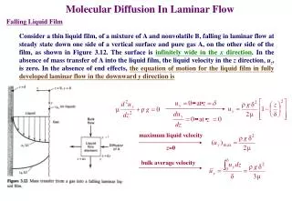
1. Molecular Diffusion In Laminar Flow Falling Liquid Film Consider a thin liquid film, of a mixture of A and nonvolatile B, falling in laminar flow at steady state down one side of a vertical surface and pure gas A, on the other side of the film, as shown in Figure 3.12. The surface is infinitely wide in the x direction. In the absence of mass transfer of A into the liquid film, the liquid velocity in the z direction, uz, is zero. In the absence of end effects, the equation of motion for the liquid film in fully developed laminar flow in the downward y direction is maximum liquid velocity z=0 bulk average velocity

2. The film thickness for fully developed flow is independent of location y and is =liquid film flow rate per unit width of film, W. For film flow, the Reynolds number, which is the ratio of the inertial force to the viscous force, is rH=hydraulic radius=(flow cross section)/(wetted perimeter) =(W)/W=  ~As reported by Grimly, for NRe < 8 to 25, depending on the surface tension and viscosity, the flow in the film is laminar and the interface between the liquid film and the gas is flat. The value of 25 is obtained with water. ~For 8 to 25 < NRe < 1,200, the flow is still laminar, but ripples and waves may appear at the interface unless suppressed by the addition of wetting agents to the liquid.

3. Consider a mole balance on A for an incremental volume of liquid film of constant density, as shown in Figure 3.12. Neglect bulk flow in the z direction and axial diffusion in the y direction. Then, at steady state, neglecting accumulation or depletion of A in the incremental volume, average concentration is L=height of the vertical surface.

4. The total rate of absorption of A from the gas into the liquid film for length L and width W is If we select cA as the driving force for mass transfer, we can write which defines a mass transfer coefficient, kc, in mol/time-area-driving force, for a concentration driving force. For the falling laminar film, we take , which varies with vertical location, y, because even though cAi is independent of y, the average film concentration, , increases with y. at the gas-liquid interface For an incremental height, we can write for film width W, an average value of kc over a length L

5. >0.1 for large  We define a Sherwood number for mass transfer, which for a falling film of characteristic length  is smallest value that Sherwood number can have for a falling liquid film The average mass transfer flux of A is given by

6. For values of <0.001, when the liquid film flow regime is still laminar without ripples, the time of contact of gas with the liquid is short and mass transfer is confined to the vicinity of the gas-liquid interface. Thus, the film acts as if it were infinite in thickness. In this limiting case, the downward velocity of the liquid film in the region of mass transfer is just uymax, We can use Fick’s first law at the gas-liquid interface to define a mass transfer coefficient with an assumption that the driving force for mass transfer in the film iscAi-cA0: an average value of kc over a length L

7. ~In the above development, asymptotic, closed-form solutions are obtained with relative ease for large and small values of . These limits, in terms of the average Sherwood number, are shown in Figure 3.13. ~The general solution for intermediate value of  is not available in closed form. Similar limiting solutions for large and small values of appropriate parameters, usually dimensionless groups, have been obtained for a large variety of transport and kinetic phenomena, as discussed by Churchill. ~Often the two limiting cases can be patched together to provide a reasonable estimate of the intermediate solution, if a single intermediate value is available from experimental or the general numerical solution. The procedure is discussed by Churchill and Usagi. The general solution of Emmert and Pigford to the falling laminar liquid film problem is included in Figure 3.13.

8. Example 3.13 Water (B) at 25 C, in contact with pure CO2 (A) at 1 atm, flows as a film down a vertical wall 1 m wide and 3 m high at a Reynolds number of 25. Using the following properties, estimate the rate of absorption of CO2 into water in kmol/s: DAB=1.9610-5 cm2/s; =1.0 g/cm3; L=0.89 cP Solubility of CO2 in ware at 1 atm and 25 C=3.410-5 mol/cm3

9. Boundary-Layer Flow on a Flat Plate Consider the flow of a fluid (B) over a thin, flat plate parallel with the direction of flow of the fluid upstream of the plate, as shown in Figure 3.14. A number of possibilities for mass transfer of another species, A, into B exist: (1)The plate might consist of material A, which is slightly soluble in B. (2)Component A might be held in the pores of an inert solid plate, from which it evaporates or dissolves into B. (3)The plate might be an inert, dense polymeric membrane, through which species A can pass into fluid B. ~Let the fluid velocity profile upstream of the plate be uniform at a free-system of velocity of uo. ~As the fluid passes over the plate, the velocity ux in the direction of flow is reduced to zero at the wall, which established a velocity profile due to drag. ~At a certain distance z, normal to and out form the solid surface, the fluid velocity is 99% of uo. This distance, which increase with increasing distance x from the leading edge of the plate, is defined as the velocity boundary-layer thickness, .

10. Essentially all flow retardation occurs in the boundary layer, as first suggested by Prandtl. The buildup of this layer, the velocity profile in the layer, and the drag force can be determined for laminar flow by solving the equations of continuity and motion (Navier-Stokes equations), for the x-direction. For a Newtonian fluid of constant density and viscosity, in the absence of pressure gradients in the x and y (normal to the x-z plane) directions, these equation for the region of the boundary layer are The solution of the above equations in the absence of heat and mass transfer, subject to these boundary conditions, was first obtained by Blasius and is described in detail by Schlicting. The result in terms of a local friction factor, fx, a local shear stress at the wall, wx, and a local drag coefficient at the wall CDx, is The thickness of the velocity boundary layer increases with distance along the plate: average values of the drag coefficient

11. A reasonably accurate expression for the velocity profile was obtained by Pohlhausen, who assumed the empirical form ux=C1z+C2z3. If the boundary conditions, ux=0 at z=0 ux=uo at z= ux/ z=0 at z= are applied to evaluate C1 and C2, the result is This solution is valid only for a laminar boundary layer that by experiment persists to NRex=5105. When mass transfer of A into the boundary layer occurs, the following continuity equation applies at constant diffusivity: If the rate of mass transfer is low, the velocity profile are undisturbed. The solution to the analogous problem in heat transfer was first obtained by Pohlhausen for NPr>0.5, as described in detail by Schlichting. The results for mass transfer are average values of the Sherwood number

12. The concentration of boundary layer, where essentially all of the resistance to mass transfer resides, is defined by and the ratio of the concentration boundary-layer thickness, c, to the velocity boundary thickness, , is Thus, for a liquid boundary layer where NSc>1, the concentration boundary layer builds up more slowly than the velocity boundary layer. For a gas boundary layer, where NSc≈1, the two boundary layers build up at about the same rate. By analogy, the concentration profile is given by

13. Example 3.14 Air at 100 C, 1 atm, and a free-stream velocity of 5 m/s flow over a 3-m-long, thin flat plate of naphthalene, causing it to sublime. (a)Determine the length over which a laminar boundary layer persists. (b)For that length, determine the rate of mass transfer of naphthalene into air. (c)At the point of transition of the boundary layer to turbulent flow, determine the thickness of the velocity and concentration boundary layers. Assume the following values for physical properties: Vapor pressure of naphthalene=10 torr Viscosity of air=0.0215cP Molar density of air=0.0327 kmol/m3 Diffusivity of naphthalene in air=0.9410-5 m2/s

14. Fully Developed Flow in a Straight, Circular Tube Figure 3.15 shows the formation and buildup of a laminar velocity boundary layer when a fluid flows from a vessel into a straight, circular tube. ~At the entrance, plane a, the velocity profile is flat. ~A velocity boundary layer then begins to buildup as shown at planes b, c and d. In this region, the central core outside the boundary layer has a flat velocity profile where the flow is accelerated over the entrance velocity. ~Finally, at plane e, the boundary layer fills the tube. From here the velocity profile is fixed and the flow is said to be fully developed. ~The distance from the plane a to plane e is the entry region. For fully developed laminar flow in a straight, circular tube, by experiment, the Reynolds number must be less than 2,100.

15. For this condition, the equation of motion in the axial direction for horizontal flow and constant properties is where the boundary conditions are The resulting equation for the velocity profile, expressed in terms of the flow-average velocity, is The shear stress, pressure drop, and Fanning friction factor are obtained: The entry length to achieve fully developed flow is defined as the axial distance, Le, from the entrance to the point at which the centerline velocity is 99% of the fully developed flow value. From the analysis of Langhaar for the entry region,

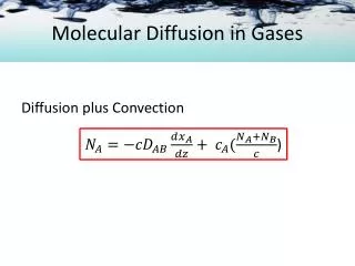
16. The species continuity equation for mass transfer, neglecting bulk flow in the radial direction and diffusion in the axial direction, is

17. Example 3.15 Lintion and Sherwood conducted experiments on the dissolution of the cast tubes of benzoic acid (A) into water (B) flowing through the tubes in laminar flow. They obtained good agreement with predictions based on the Graetz and Leveque equations. Consider a 5.23-cm-inside-diameter by 32-cm-long tube of benzoic acid, preceded by 400 cm of straight metal pipe of the same inside diameter where a fully developed velocity profile is established. Pure water enters the system at 25 C at a velocity corresponding to a Reynolds number of 100. Based on the following property data at 25 C, estimate the average concentration of benzoic acid in the water leaving the cast tube before a significant increase in the inside diameter of the benzoic acid tube occurs because of dissolution. Solubility of benzoic acid in water=0.0034 g/cm3 Viscosity of water=0.89 cP=0.0089 g/cm-s Diffusivity of benzoic acid in water at infinite dilution=9.1810-6 cm2/s

18. Mass Transfer In Turbulent Flow Reynolds Analogy Define dimensionless velocity and solute concentration by It can be used to estimate values of mass transfer coefficients from experimental measurements of the Fanning friction factor for turbulent flow, but only when NSc=1.

19. Chilton-Colburn Analogy 1.Flow through a straight, circular tube of inside diameter D: 2.Average transport coefficients for flow across a flat plate of length L: 3.Average transport coefficients for flow normal to a long circular cylinder of diameter D, where the drag coefficient includes both form drag and skin friction, but only the skin friction contribution applies to the analogy:

20. 4.Average transport coefficient for flow past a single sphere of diameter D: 5.Average transport coefficient for flow through beds packed with spherical particles of uniform size D: NSc is evaluated at the average conditions from the surface to the bulk stream.

21. Prandtl Analogy Prandtl divided the flow into two regions: (1) a thin laminar sublayer of thickness  next to the wall boundary, where only molecular transport occurs (2) a turbulent region dominated by eddy transport, with M=D. simplify to the Reynolds analogy when NSc=1

22. Example 3.16 Linton and Sherwood conducted experiments on the solution of cast tubes of cinnamic acid (A) into water (B) flowing through the tubes in the turbulent flow. In one run, with a 1.90-cm-i.d tube, NRe=62,000, and NSc=3,000, they measured a Stanton number for mass transfer, NSt, of 0.0000136. Compare this experimental value with predictions by the Reynolds, Chilton-Colburn, and Prandtl analogies. Solution Reynolds Analogy Chilton-Colburn Analogy Prandtl Analogy