A Quick Algorithm for Knowledge Reduction Based on Quick Sort
A Quick Algorithm for Knowledge Reduction Based on Quick Sort. Feng Hu, Guoyin Wang, Lin Feng Institute of Computer Science and Technology, Chongqing University of Posts and Telecommunications, Chongqing, 400065, China. Contents. Introduction Quick Sort for Two Dimension Table


A Quick Algorithm for Knowledge Reduction Based on Quick Sort
E N D
Presentation Transcript
A Quick Algorithm for Knowledge Reduction Based on Quick Sort Feng Hu, Guoyin Wang, Lin Feng Institute of Computer Science and Technology, Chongqing University of Posts and Telecommunications, Chongqing, 400065, China
Contents • Introduction • Quick Sort for Two Dimension Table • Complexity Analysis of Quick Sort Algorithm • Experiment Results of Quick Sort • Quick Reduction Algorithm Based on Attribute Order • Complexity Analysis of Reduction Algorithm • Experiment Results of Reduction Algorithm • Conclusions and Future Works
1. Introduction • The problem of processing huge data sets has been studied for many years. Many valid technologies and methods for dealing with this problem have been developed.
1. Introduction (contl.) Some Valid Methods Have Been Proposed. In 1991, Carlett J proposed Random sampling method, but the method can not work when number of samples is over 32000. In 1996, Philip K C divided a big data set into some subsets which fit in memory at first, and then developed a classifier for each subset in parallel. However, its accuracy is less than those processing a data set as a whole. In 1996, IBM Almaden Research Center developed SLIQ and SPRINT. They can be used to process with disk-resident data directly. In 1998, by impoving SLIQ and SPRINT, Alsabti K and Ranka S proposed CLOUDS, and Joshi M and Karypis G propoed ScalParC. In 1998, Gehrke J and Ramkrishnan R proposed RainForest. It is a framework for fast decision tree construction for large datasets. Its speed and effect are better than SPRINT in some cases. In 2002, Ren L A, He Q and Shi Z Z used hyper surface separation and HSC classification method to classify huge data sets and achieved a good performance.
1. Introduction • Rough Set (RS) is a valid mathematical theory to deal with imprecise, uncertain, and vague information. It has been applied in such fields as machine learning, data mining, intelligent data analyzing and control algorithm acquiring, etc, successfully since it was proposed by Professor Z. Pawlak in 1982.
1. Introduction • Attribute reduction is a key issue in rough set theory. In recent years, many researchers have proposed many algorithms for computing attribute reduction. • Attribute reduction algorithms can be divided into two categories: (1) Reduction without attribute order. (2) Reduction based on attribute order.
1. Introduction (contl.) Attribute Reduction Algorithms without Attribute Order. In 1992, Skowron proposed an algorithm for attribute attribute based discernibility matrix. It’s time complexity is , space complexity is . In 1995, Hu X H improved Skowron’s algorithm and proposed a new algorithm for attribute attribute with complexities . In 1996, Nguyen proposed an algorithm for attribute reduction by sorting decision table. It’s complexities are In 2002, Wang G Y proposed an algorithm for attribute reduction based on information entropy. It’s complexities are In 2003, Liu S H proposed an algorithm for attribute reduction by sorting and partitioning universe. It’s complexities are
1. Introduction (contl.) Attribute Reduction Algorithms Based on Attribute Order. In 2001, using Skowron’s discernibility matrix, Wang J proposed an algorithm for attribute reduction based on attribute order. Its complexity are t=O(m×n2), s=O(m×n2) (m>>n). In 2004, Zhao M and Wang J proposed an algorithm for attribute reduction with tree structure based on attribute order. Its complexity are t=O(m2×n), s=O(m×n) (m<<n).
1. Introduction (contl.) • Quick sort for two dimension table is an important operation in data mining. • In huge data base processing based on rough set theory, it is a basic operation to divide a decision table into indiscernible classes. • Many researchers deal with this problem using the quick sort method.
1. Introduction (contl.) Suppose that the data of a two dimension table is in uniform distribution. • Many researchers think that the average time complexity of quick sort for a two dimension table with m attributes and n objects is O(n×logn×m) . • Thus, the average time complexity for computing the positive region of a decision table will be no less than O(n×logn×m) . • However, we find that the average time complexity of sorting a • two dimension table is O(n×(logn+m)) .
1. Introduction (contl.) • Divide and Conquer Method It divides a complex problem into simpler sub-problems with same structures iteratively and at last the sizes of the sub-problems will become small enough to be processed directly. • Quick sort is a typical divide and conquer method.
1. Introduction (contl.) Since the time complexity of sorting a two dimension table (m attributes, n objects) is O(n×(m+logn)), and quick sort is a divide and conquer method, we may improve reduction methods of rough set theory.
2. Quick Sort for Two Dimension Table • Firstly, an example is discussed to show the process of sorting a two dimension table. • Secondly, a quick sort algorithm for two dimension table (m attributes, n objects) is proposed. • Thirdly, the time complexity and space complexity of the algorithm is analyzed.
U k1 k2 k3 k4 U k2 k3 k4 S1 x1 2 3 2 2 x3 1 0 2 x2 2 3 1 3 x5 1 0 1 Sort on k1 x3 0 1 0 2 S U k2 k3 k4 x4 1 2 2 0 S2 x4 2 2 0 x5 0 1 0 1 U k2 k3 k4 x1 3 2 2 S3 x2 3 1 3 An example of sorting a two dimension table
U k2 k3 k4 U k3 k4 U k4 U k4 Sort on k2 Sort on k3 Sort on k4 S1 x3 1 0 2 x3 0 2 x3 2 x5 1 x5 1 0 1 x5 0 1 x5 1 x3 2 U k2 k3 k4 Only one object, return. S2 x4 2 2 0 U k3 k4 x2 1 3 U k3 k4 U k2 k3 k4 Sort on k2 Sort on k3 x1 2 2 S3 x1 3 2 2 U k3 k4 x2 1 3 x2 3 1 3 x1 2 2 An example of sorting a two dimension table
Quick Sort Algorithm for Two Dimension TableAlgorithm 1 • Input: A two dimension table S[1..n][1..m]. • Output: An ordered table S[1..n][1..m]. • Step1: for i=1 to n do • L[i]=i ;(L[1..n] is an temporary array) • end for • Step2:TwoDimension_QuickSort (1, 1, n ); • Step3: Return S.
procedureTwoDimension_QuickSort (intr, intlow, inthigh ) if( r > m ) thenreturn; if(low = high) thenreturn; boolCanBePartition = false; forj = low+1 tohigh do { if (S[L[j]][r]≠S[L[low]][r]) then { CanBePartition = true ; break;}} if ( CanBePartition = = true ) then {intaverage= (S[L[low]][r]+S[L[(low+high)/2]][r]+S[L[high]][r])/3; intmid = callPartition (r, low, high , average); callTwoDimension_QuickSort (r, low, mid ); callTwoDimension_QuickSort (r, mid +1, high ); } else callTwoDimension_QuickSort (r + 1 , low, high ); endTwoDimension_QuickSort
T0 T1 T2 3. Complexity Analysis of Quick Sort Algorithm • The time complexity can be approximated by the following recursive equation:
T0 represents the total time cost of calling recursive expressions (a) and (b), • T1 represents the total time cost of calling recursive expression (c), • T2 represents the total time cost of calling recursive expression (d). T=T0+T1+T2. (1) Both the average and worst time cost of T1is O(m×n). (2) Now, we analyze the time complexity of (T0+T2) The time cost of (T0+T2) can be approximate by the following recursive equation.
T1(n) is the same as the time complexity equation of quick sort on a one-dimension array. When the data obey the uniform distribution, T1(n) is O(n×logn). Therefore, the average time complexity of Algorithm 1 is : T(n, r) = T1+ (T0 + T2) = T1+ T1(n) = O(n×m) + O(n×logn) = O(n×(m + logn))
Analysis of Space Complexity • Suppose s be the space complexity of Algorithm 1, s(r,n) be its stack space complexity. Then, s(r,n) can be approximated by the following recursive equation. We can find, Because the array L[1..n] takes O(n) space, thus
4. Experiment Results of Quick Sort • Experiment Steps: • At first, the number of records (n) is fixed, Algorithm 1 is tested by adding attributes (m) step by step. (n>>m) • Secondly, the number of attributes (m) is fixed, Algorithm 1 is tested by adding records (n) step by step. (m>>logn).
Experiment Results (n>>m) • Number of data sets: 100 (There are 10 groups of data sets). • n: number of records (×105). • m: number of attributes (×2). • Experiment environment: P4 2.6G CPU, 256M RAM, Windows XP. T is not linear with m!
Experiment Results (m>>logn) • Number of data sets: 20. • n: number of records (×500). • m: number of attributes (m=200). • Experiment environment: P4 2.6G CPU, 256M RAM, Windows XP. T is linear with n approximately.
5. Quick Attribute Reduction Algorithm Based on Attribute Order • Firstly, an algorithm for computing the non-empty label attribute set of a decision table is developed. • Secondly, a quick algorithm for attribute reduction based on attribute order is developed. • Thirdly, an example of our algorithm is discussed.
Non-empty Label Attribute • Let be a decision table, we define an attribute order relation over C: • Suppose M is the discernibility matrix of S. , the attribute of inherit the order relation of SO from left to right. i.e. , B is a subset of C. aj will be the first attribute of in SO. aj is called the label attribute of .
x1 x2 x3 x4 x5 S x1 c1,c3,c4 c1,c2,c3,c4 c1,c2,c3,c4 U c1 c2 c3 c4 d x1 1 2 2 1 1 discernibility matirx c1,c3,c4 c1,c2,c3 c2,c3,c4 x2 x2 1 0 3 0 0 x3 2 1 0 1 0 c1,c2,c3,c4 c3,c4 x3 x4 2 1 1 0 1 x5 1 2 2 1 0 c1,c2,c3,c4 c1,c2,c3 c3,c4 c1,c2,c3,c4 x4 x5 c2,c3,c4 c1,c2,c3,c4 c4: Example for Non-empty Label Attributes c1:{{c1,c2,c3}, {c1,c2,c3,c4}, {c1,c3,c4}} c2:{ {c2,c3,c4}} c3:{ {c3,c4}} c1,c2,c3are non-empty label attributes.
S U c1 c2 c3 c4 d (1) In S, x1 1 2 2 1 1 x2 1 0 3 0 0 x3 2 1 0 1 0 U c2 c3 c4 d U c2 c3 c4 d x4 2 1 1 0 1 x1 2 2 1 1 x3 1 0 1 0 S1 + S2 x5 1 2 2 1 0 x2 0 3 0 0 x4 1 1 0 1 x5 2 2 1 0 U c3 c4 d S3 x2 3 0 0 (2) In S1, U c3 c4 d x1 2 1 1 S4 x5 2 1 0 (4) In S4, ,return Example for Computing Non-empty Label Attributes (3) In S3, |U|=1, return
(5) In S2, S2 (6) In S5, U c2 c3 c4 d U c3 c4 d S5 x3 1 0 1 0 x3 0 1 0 x4 1 1 0 1 x4 1 0 1 U c4 d U c4 d S6 S7 x3 0 1 x3 1 0 Example for Computing Non-empty Label Attributes (7) In S6, |U|=1, return; (8) In S7, |U|=1, return; Therefore, R1={c1,c2,c3}
Algorithm for Computing Non-empty Label Attributes Algorithm 2 Input: A decision table and attribute order Output: The non-empty label attribute set of S Step1: For j = 1 to |C| do NonEmptyLabel [j] = 0 ; Step2: NonEmptyLabelAttr (1, ); Step3: For j = 1 to |C|do IfNonEmptyLabel [j] = 1 then Step4: Return .
VoidNonEmptyLabelAttr (intr, ObjectSetOSet) { Ifr<|C|+1 then { If |OSet|=1, then return ; ElseIf POSC(D)=Φ, thenreturn; ElseIf |V(cr)|=1, then { r = r+1; NonEmptyLabelAttr (r, OSet) ; } Else { NonEmptyLabel [r] = 1 ; Divide OSet into |V(cr)| parts: ; r=r+1; for (i=1; i<|V(cr-1)|+1; i++) NonEmptyLabelAttr (r , ) ; } } }
Quick Attribute Reduction Algorithm Based on Attribute Order Algorithm 3 Input: A decision table and Output: Attribute Reduction of table S Step1: Step2: Computing positive region . Step3: Computing non-empty label attribute set by Algorithm 2. Step4: Suppose be the maximum label attribute of . R; If , Then return R; Else Given new attribute order: Computing new non-empty label attribute set by Algorithm 2. Go to Step4.
S (1) (2) U c1 c2 c3 c4 d x1 1 2 2 1 1 (3) x2 1 0 3 0 0 x3 2 1 0 1 0 x4 2 1 1 0 1 U c3 c1 c2 d x5 1 2 2 1 0 x1 2 1 2 1 S1 x2 3 1 0 0 Because x3 0 2 1 0 x4 1 2 1 1 Thus, return x5 2 1 2 0 Example of Algorithm 3
6. Complexity Analysis of Reduction Algorithm In Algorithm 3, In Step2, average time complexity: O(n×m). space complexity: O(n). In Step3, average time complexity: O(n×(m+logn)). space complexity: O(m+n). In Step4, average time complexity: (m×n×(m+logn)). space complexity: O(m+n). In total, time complexity: O(m×n×(m+logn)) space complexity: O(m+n).
7. Experiment Results of Reduction Algorithm • Experiment Steps: • At first, KDDCUP99 data sets(huge data sets) are used to test Algorithm 3. (Data set KDDCUP99 can be downloaded at http://kdd.ics.uci.edu/databases/kddcup99/kddcup99.html). • Secondly, random data sets are generated. The data sets are used to test Algorithm 3 (n >> m). • Thirdly, random data sets are generated. The data sets are used to test Algorithm 3 (n << m).
n m T N MemUse 489843 41 61.232417 29 198804 979686 41 135.023143 30 246972 1469529 41 218.743598 31 303232 1959372 41 283.406260 30 344984 2449216 41 384.723173 30 395144 2939059 41 469.103032 32 444576 3428902 41 602.920099 34 493672 3918745 41 661.663162 33 543172 4408588 41 753.895816 33 592372 4898432 41 13337.205877 34 641896 Experiment Results(KDDCUP99) • T: running time of Algorithm 3(Unit: second). m: number of attributes. • n: number of records. N: number of reduction attributes. • MemUse: Occupied maximum memory when Algorithm 3 runs(Unit: KB). • Experiment environment: P4 2.6G CPU, 512M RAM, Windows XP.
Experiment Results(KDDCUP99) Running Time(Unit: Second) MemUse(Unit: KB) Number of Records(Unit: 489843) Number of Records(Unit: 489843)
Experiment Results(n>>m) • Number of data sets: 30. • Number of condition attributes is 15. • Experiment environment: P4 2.6G CPU, 256M RAM, Windows XP. Running Time(Unit: Second) Number of Records(Unit: 105)
Experiment Results(m>>n) • Number of data sets: 10. • Number of records is 1000. • Experiment environment: P4 2.6G CPU, 256M RAM, Windows XP. Running Time(Unit: Second) Number of condition attributes(Unit: )
Conclusions • By analyzing and experiments, we find that the average time complexity of quick sorting a two dimension table (m keys, n records) is O(n×(m+logn)). The space complexity is O(n). • If m>>logn, the time complexity of quick sorting two dimension table is O(n×m)approximately • Given an attribute order, we proposed a quick attribute reduction algorithm for decision table. Its time complexity is O(m×n×(m+logn)). Its space complexity is O(m+n). • The reduction algorithm proposed can process huge data bases quickly.
Original data set Future Works Get sample recognizing result. Recognizing Rule acquisition Extract unique rule set based on attribute order. Aim: process (106×41) within 10 minute. t=O(m×n×(m+logn)), s=O(m×n) Generate attribute reduction based on attribute Order. Aim: process (106×41) within 5 minute. t=O(m×n×(m+logn)), s=O(m+n) Attribute reduction Discrete Generate discretised data sets based attribute order. Aim: process (106×41) within 10 minute. t=O(n×(m+logn)), s=O(m+n) Attribute order is used.
Original data set Future Works Get sample recognizing result. Recognizing Rule acquisition Extract unique rule set based on attribute order. Aim: process (106×41) within 10 minute. t=O(m×n×(m+logn)), s=O(m×n) Generate attribute reduction based on attribute Order. Aim: process (106×41) within 5 minute. t=O(m×n×(m+logn)), s=O(m+n) Attribute reduction Completed Discrete Generate discretised data sets based attribute order. Aim: process (106×41) within 10 minute. t=O(n×(m+logn)), s=O(m+n) Attribute order is used.
Future Works (Contl.) Original data sets Get sample recognizing result. Recognizing Extract rule set. Aim: process (106×41) within 10 minute. t=O(m×n×(m+logn)), s=O(m×n) Rule acquisition Get complete Pawlak attribute reduction. Aim:process (106×41) within 30 minute. t=O(m×n×(m+logn)), s=O(m+n) Attribute reduction Generate attribute cores. Aim: process (106×41) within 30 minute. t=O(n×m2), s=O(m+n) Computing attribute core Discrete Generate discretised data sets. Aim: process (106×41) within 10 minute. t=O(n×(m+logn)), s=O(m+n) Attribute order is not used.
Future Works (Contl.) Original data sets Get sample recognizing result. Recognizing Extract rule set. Aim: process (106×41) within 10 minute. t=O(m×n×(m+logn)), s=O(m×n) Rule acquisition Get complete Pawlak attribute reduction. Aim:process (106×41) within 30 minute. t=O(m×n×(m+logn)), s=O(m+n) Attribute reduction We have solved it. The algorithm can process (106×41) within 30 minute. t=O(n×m2), s=O(m+n). Computing attribute core Completed Discrete Generate discretised data sets. Aim: process (106×41) within 10 minute. t=O(n×(m+logn)), s=O(m+n) Attribute order is not used.