Understanding Recurrent Neural Networks for Pattern Recognition
Learn about recurrent networks & their applications in pattern recognition. Explore examples, encoding methods & Hopfield networks. Discover update strategies, neighborhood & convergence in network states.

Understanding Recurrent Neural Networks for Pattern Recognition
E N D
Presentation Transcript
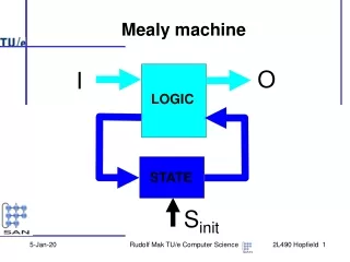
Mealy machine O I LOGIC STATE Sinit Rudolf Mak TU/e Computer Science
I LOGIC STATE LOGIC O Sinit Moore machine Rudolf Mak TU/e Computer Science
FFNN Recurrent Neural Net y STATE x Rudolf Mak TU/e Computer Science
Recurrent Networks • A recurrent network is characterized by • The connection graph of the network has cycles, i.e. the output of a neuron can influence its input • There are no natural input and output nodes • Initially each neuron has a given input state • Neurons change state using some update rule • The network evolves until some stable situation is reached • The resulting state is the output of the network Rudolf Mak TU/e Computer Science
Pattern Recognition • Recurrent networks can be used for pattern • recognition in the following way: • The stable states represent the patterns to • be recognized • The initial state is a noisy or otherwise • mutilated version of one of the patterns • The recognition process consists of the • network evolving from its initial state to a • stable state Rudolf Mak TU/e Computer Science
Pattern Recognition Example Rudolf Mak TU/e Computer Science
Pattern Recognition Example (cntd) Noisy image Recognized pattern Rudolf Mak TU/e Computer Science
Bipolar Data Encoding • In bipolar encoding firing of a neuron is repre-sented by the value 1, and non-firing by the value –1 • In bipolar encoding the transfer function of the neurons is the sign function sgn • A bipolar vector x of dimension n satisfies the equations • sgn(x) = x • xTx = n Rudolf Mak TU/e Computer Science
Binary versus Bipolar Encoding • The number of orthogonal vector pairs is much • larger in case of bipolar encoding. In an even n- • dimensional vector space: • For binary encoding • For bipolar encoding Rudolf Mak TU/e Computer Science
Hopfield Networks • A recurrent network is a Hopfield network when • The neurons have discrete output (for conve-nience we use bipolar encoding, i.e., activation function is the sign function) • Each neuron has a threshold • Each pair of neurons is connected by a weighted connection. The weight matrix is symmetric and has a zero diagonal (no connection from a neuron to itself) Rudolf Mak TU/e Computer Science
Network states If a Hopfield network has n neurons, then the state of the network at time t is the vector x(t) 2 {-1, 1}n with components x i (t) that describe the states of the individual neurons. Time is discrete, so t2N The state of the network is updated using a so-called update rule. (Not) firing of a neuron at time t+1 will depend on the sign of the total input at timet Rudolf Mak TU/e Computer Science
Update Strategies • In a sequential network only one neuron at a time is allowed to change its state. In the asyn-chronous update rule this neuron is randomly selected. • In a parallel network several neurons are allowed to change their state simultaneously. • Limited parallelism: only neurons that are not connected can change their state simultaneously • Unlimited parallelism: also connected neurons may change their state simultaneously • Full parallelism: all neurons change their state simul-taneously Rudolf Mak TU/e Computer Science
Asynchronous Update Rudolf Mak TU/e Computer Science
Asynchronous Neighborhood The asynchronous neighborhood of a state x is defined as the set of states Because wkk = 0 , it follows that for every pair of neighboring states x*2Na(x) Rudolf Mak TU/e Computer Science
Synchronous Update This update rule corresponds to full parallelism Rudolf Mak TU/e Computer Science
Sign-assumption In order for both update rules to be applica-ble, we assume that for all neurons i Because the number of states is finite, it is always possible to adjust the thresholds such that the above assumption holds. Rudolf Mak TU/e Computer Science
Stable States A state x is called a stable state, when For both the synchronous and the asyn-chronous update rule we have: a state is a stable state if and only if the update rule does not lead to a different state. Rudolf Mak TU/e Computer Science
1 1 1 -1 1 -1 -1 1 1 Cyclic behavior in asymmetric RNN 1 1 -1 -1 -1 1 Rudolf Mak TU/e Computer Science
Basins of Attraction stable state initial state state space Rudolf Mak TU/e Computer Science
Consensus and Energy The consensus C(x) of a state x of a Hopfield network with weight matrix W and bias vector b is defined as The energy E(x) of a Hopfield network in state x is defined as Rudolf Mak TU/e Computer Science
Consensus difference For any pair of vectors x and x* 2Na(x) we have Rudolf Mak TU/e Computer Science
Asynchronous Convergence If in an asynchronous step the state of the network changes from x to x-2xkek, then the consensus increases. Since there are only a finite number of states, the consensus serves as a variant function that shows that a Hopfield network evolves to a stable state, when the asynchronous update rule is used. Rudolf Mak TU/e Computer Science
Stable States and Local maxima A state x is a local maximum of the consensus function when Theorem: A state x is a local maximum of the consensus function if and only if it is a stable state. Rudolf Mak TU/e Computer Science
Stable equals local maximum Rudolf Mak TU/e Computer Science
Modified Consensus The modified consensus of a state x of a Hopfield network with weight matrix W and bias vector b is defined as Let x,x*, and x** be successive states obtained with the synchronous update rule. Then Rudolf Mak TU/e Computer Science
Synchronous Convergence Suppose that x, x*, and x** are successive states obtained with the synchronous update rule. Then Hence a Hopfield network that evolves using the synchronous update rule will arrive either in a stable state or in a cycle of length 2. Rudolf Mak TU/e Computer Science
Storage of a Single Pattern How does one determine the weights of a Hopfield network given a set of desired sta- ble states? First we consider the case of a single stable state. Let x be an arbitrary vector. Choos-ing weight matrix W and bias vector b as makes x a stable state. Rudolf Mak TU/e Computer Science
Proof of Stability Rudolf Mak TU/e Computer Science
Hebb’s Postulate of Learning • Biological formulation • When an axon of cell A is near enough to excite a cell and repeatedly or persistently takes part in firing it, some growth process or metabolic change takes place in one or both cells such that A’s efficiency as one of the cells firing B is increased. • Mathematical formulation Rudolf Mak TU/e Computer Science
Hebb’s Postulate: revisited • Stent (1973), and Changeux and Danchin (1976) • have expanded Hebb’s rule such that it also mo- • dels inhibitory synapses: • If two neurons on either side of a synapse are activated simultaneously (synchronously), then the strength of that synapse is selectively increased. • If two neurons on either side of a synapse are activated asynchronously, then that synapse is selectively weakened or eliminated. Rudolf Mak TU/e Computer Science
Example Rudolf Mak TU/e Computer Science
State encoding Rudolf Mak TU/e Computer Science
Finite state machine for async update Rudolf Mak TU/e Computer Science
Weights for Multiple Patterns Let {x(p)j 1 ·p·P } be a set of patterns, and let W(p) be the weight matrix corresponding to pattern number p. Choose the weight matrix W and the bias vector b for a Hopfield network that must recognize all P patterns as Question: Is x(p) indeed a stable state? Rudolf Mak TU/e Computer Science
Remarks • It is not guaranteed that a Hopfield network with weight matrix as defined on the previous slide indeed has the patterns as it stable states • The disturbance caused by other patterns is called crosstalk. The closer the patterns are, the larger the crosstalk is • This raises the question how many patterns there can be stored in a network before crosstalk gets the overhand Rudolf Mak TU/e Computer Science
Weight matrix entry computation Rudolf Mak TU/e Computer Science
Input of neuron i in state x(p) Rudolf Mak TU/e Computer Science
Neuron i is stable when , because Crosstalk The crosstalk term is defined by Rudolf Mak TU/e Computer Science
Spurious States • Besides the desired stable states the network can • have additional undesired (spurious) stable states • If x is stable and b=0, then –x is also stable. • Some combinations of an odd number of stable states can be stable. • Moreover there can be more complicated additional stable states (spin glass states) that bare no relation to the desired states. Rudolf Mak TU/e Computer Science
Storage Capacity Question: How many stable states P can be stored in a network of size n ? Answer: That depends on the probability of instability one is willing to accept. Experi- mentally P¼ 0.15n has been found (by Hopfield) to be a reasonable value. Rudolf Mak TU/e Computer Science
Then it can be shown that has ap- proximately the standard normal distribu- tion N(0, 1). Probabilistic analysis 1 Assume that all components of the patterns are random variables with equal probability of being 1 and -1 Rudolf Mak TU/e Computer Science
Normal distribution Rudolf Mak TU/e Computer Science
Probabilistic Analysis 2 From these assumptions it follows that Application of the central limit theorem yields Rudolf Mak TU/e Computer Science
Standard Normal Distribution The shaded area under the bell-shaped curve gives the probability Pr[y¸ 1.5] Rudolf Mak TU/e Computer Science
Probability of Instability Rudolf Mak TU/e Computer Science
Topics Not Treated • Reduction of crosstalk for correlated patterns • Stability analysis for correlated patterns • Methods to eliminate spurious states • Continuous Hopfield models • Different associative memories • Binary Associative Memory (Kosko) • Brain State in a Box (Kawamoto, Anderson) Rudolf Mak TU/e Computer Science