Optimal Pricing and Return Policies for Perishable Commodities B. A. Pasternack
450 likes | 723 Vues
Optimal Pricing and Return Policies for Perishable Commodities B. A. Pasternack. Presenter: Gökhan METAN. Outline. Introduction Model Implications Examples Conclusion. Introduction. What the paper is all about?

Optimal Pricing and Return Policies for Perishable Commodities B. A. Pasternack
E N D
Presentation Transcript
Optimal Pricing and Return Policies for Perishable CommoditiesB. A. Pasternack Presenter: Gökhan METAN Pasternack
Outline • Introduction • Model • Implications • Examples • Conclusion Pasternack
Introduction What the paper is all about? Pricing policies for a manufacturer that produceses goods with short shelf or demand life. Pricing Policy: Specifies the price of the commodity charged from the retailers, per unit credit for the returned goods, and the percentage of purchased goods allowed to be returned for this credit. Pasternack
Introduction Question: How would you set the price of the product for your retailers, and what return policy would you impose? How and what kind of decisions are made typically? Price: i- Cost basis decisions ii- “What market will bear” approach Return Policy: i- Full credit for all unsold goods. ii- No credit for unsold goods. No channel coordination! Pasternack
Profit Profit Introduction Set a pricing policy Purchase Decision Customer Side Price, demand, product availability Pasternack
Introduction Assumptions about the model: i- Single item is considered. ii- Item has short shelf or demand life. iii- Any retailer place only one order from the manufacturer. iv- Goodwill cost is incurred partially by the retailer and partially by the manufacturer. (when inventory is depleated) v- Certain amount may be returned to the manufacturer for partial credit and the remaining is disposed of by the retailer for its salvage value. (when inventory remains beyond the shelf/demand life) Pasternack
Introduction Assumptions about the model: Cont’d vi- Manufacturing cost per item is independent of the production quantity. vii- All the retailers charge the same (fix) price for the product. viii- Both the manufacturer and the retailers are profit maximizers. ix- Salvage value is same for manufacturer and the retailers. x- No transfer mark-ups between retailers and the manufacturer. (amount paid by the retailer = amount received by the manufacturer) Pasternack
Objective: To develop a pricing policy that optimizes the expected profit of both the manufacturer and the retailers as well as to achieve the channel coordination. Introduction Assumptions about the model: Cont’d xi- Demand at the retail level is stochastic. xii- Manufacturer has control of the channel and is free to set the pricing policy. Retailers decide to carry the commodity or not. Pasternack
Introduction Methodology: Single period inventory model (newsboy problem) is employed in the analyses. Interest: Not finding the optimal ordering quantity! What pricing policy for the manufacturer will be optimal ? Pasternack
Model Pasternack
Manufacturing cost per item Unit selling price by the retailer Unit price paid by the retailer to the manufacturer. Salvage value per unit Manufacturing cost per item Model Pasternack
This will enable us to determine the optimal policy for the system as a whole. This will enable us to determine the optimal policy for retailers where they are independent. Model In the analyses we will consider two cases: 1) We will first assume such a system that the retailers belong to manufacturers own. That is, they are company stores. 2) In the second case, we will consider indedendent retailers. That is, the retailers determine their order quantity. Pasternack
Total manufacturing cost Total Profit Total Profit Expected profit when demand is more than the production quantity. Total goodwill cost for lost demands Expected profit when demand is less than the production quantity. Total Salvage Value for unsold goods Model 1st CASE Let the company produces Qunits and sells directly to the customers by its own retailers and EPT(Q) be the total expected profit. Pasternack
Model Result F(QT*)=(p+g2-c)/(p+g2-c3) Pasternack
Model Retailer’s total ordering cost 2nd CASE Let the retailer orders Qunits and EPR(Q) be the retailer’s expected profit. Pasternack
Q ORDER DEMAND 0 x (1-R)Q Retailer’s revenue from items sold Credit obtained for unsold goods from the manufacturer Total amount obtained for unsold goods from their salvage value Model RQ Pasternack
x Credit obtained for unsold goods from the manufacturer Retailer’s revenue from items sold Model Q ORDER DEMAND 0 RQ (1-R)Q Pasternack
x Total goodwill cost of the retailer. Retailer’s revenue from items sold Model Q ORDER DEMAND 0 RQ (1-R)Q Pasternack
0 0 Model Note that: Q* is the order quantity of independent retailer which satisfies equation (7). Pasternack
Profit obtained by the sales of Q* units to the retailer Model Now, the retailer orders Q*units and EPM(Q*) be the manufacturer’s expected profit. Pasternack
Q* ORDER DEMAND 0 x (1-R)Q* Total Credit paid for returned unsold goods minus the total salvage value obtained from these items by the manufacturer Model RQ* Pasternack
x Total Credit paid for returned unsold goods minus the total salvage value obtained from these items by the manufacturer Model Q* ORDER DEMAND 0 RQ* (1-R)Q* Pasternack
x Total goodwill cost of the manufacturer (because of lost demand) Model Q* ORDER DEMAND 0 RQ* (1-R)Q* Pasternack
We know that the independent retailer wants to maximize its own profit and hence wants: Q* such that it satisfies: Model Now what we have on hand? From Case-1 Analysis: We know that the manufacturer wants to maximize the total channel profit and hence wants: QT* such that it satisfies F(QT*)=(p+g2-c)/(p+g2-c3) From Case-2 Analysis: Pasternack
Model Hence set: Q*=QT* such that it satisfies F(Q*)=F(QT*)=(p+g2-c)/(p+g2-c3) Pasternack
Results: • If the manufacturer sets these three parameters in such a way that the previous equation is satisfied, the independent retailer should order the same quantity from the manufacturer as would the manufacturer if operating a company store. • This results in maximum total profits to the retailer and manufacturer, and the channel is said to be coordinated. Model The manufacturer has the control over the parameters c1 (cost of per unit order from the manufacturer), c2 (credit per unit paid by the manufacturer to the retailer for returned goods) and R (percentage of the order quantity, Q, that can be returned to the manufacturer for a credit of c2 per item). • Observations: • As there is no unique solution to the previous equation, different values for these there decision variables result in different divisions of expected profit between the manufacturer and the retailer. • Therefore, the manufacturer’s pricing and return policy will function as a risk sharing agreement between manufacturer and retailer. Pasternack
Implications Theorem 1. The policy of a manufacturer allowing unlimited returns for full credit is system suboptimal. Pasternack
Implications Theorem 2. The policy of a manufacturer allowing no returns is system suboptimal. Theorems 1 & 2 imply that “unlimited returns for full credit” as well as “no returns” prevents channel coordination. Theorem 3. A policy which allows for unlimited returns (R=1) at partial credit (c2<c1) will be system optimal for appropriately chosen values of c1 and c2. Pasternack
Implications If c1 and c2 are so chosen and the manufacturer allows for unlimited returns, then the total expected profit for the retailer and manufacturer are as follows: Pasternack
Implications If the demand for the commodity follows a normal distribution (x ~ N(μ, σ)) then the previous equations become: OBSERVATIONS: c1 chosen at its low end (c1 = c + ε) Manufacturer makes NO PROFIT c1 chosen at its high end (c1 =p – ε) Retailer makes NO PROFIT Pasternack
As c2 ↑ c1 also ↑ Implications Pasternack
Results & Suggestions: Implications If it can be demonstrated to the retailers that their profits will improve as a result of price changes, then they should be more willing to accept the new pricing plan. REASON Increasing the retailers’ profits should result in additional distribution outlets being opened, resulting in an increase in overall demand. The pricing should be set so that the average retail establishment captures at least some portion of the gain from channel coordination. Pasternack
Results & Suggestions: Implications A drawback!!! Multi-retailer Environment Manufacturer sets a single (uniform) pricing policy for all retailers Impacts on retailer profitability will be different An easy but not feasible solution: A different and retailer-specific pricing policy can be determined and set for each retailer and this achieves the manufacturer’s goal. In fact it is not defendable under the Robinson-Patman Act (which is an act about the competition and pricing actions in business environment). A policy that increases retailers’ total profit does not guarantee to increase all individual retailer’s profit. Some may faced with a decrease in their expected profit due to the channel coordinated pricing policy. Pasternack
Results & Suggestions: Implications Ensure reasonable rate of return $$$$$$ A pricing policy for a new product! Desirable enough $$$ Another issue Goodwill Costs Hard to Quantify Vary among different retailers A uniform pricing policy for those retailer can not be set Fortunately, analyses show that when R=0 the retailers’ order quantity is insensitive to small changes in goodwill cost. Pasternack
Examples Consider a product with: Net retail price of $8.00 (p=8). Manufacturing cost of $3.00 (c=3) Salvage value of $1.00 (c3=1) Retailer goodwill cost is $3.00 (g=3) Manufacturer goodwill cost is $2.00 (g1=2) Total goodwill cost is $5.00 (g2=g+g1=5) Suppose that manufacturer charges $4.00 (c1=4) per item from the retailer and not permit returns for unsold goods (R=0). g=3, g1=2, g2=5, p=8, c=3 , c1=4, c3=1, R=0 Pasternack
Examples g=3, g1=2, g2=5, p=8, c=3 , c1=4, c3=1, R=0 Assume a retailer: Demand ~ N(200, 50) and the retailer is a profit maximizer. Q*=226 EPR(Q*)=$626.25 EPM(Q*)=$206.85 (1) From Theorem-2, this cannot be optimal! Manufacturer decides to allow unlimited returns to achieve channel coordination. Set R=1. Pasternack
Examples g=3, g1=2, g2=5, p=8, c=3 , c1=4, c3=1, R=1 From F(QT*)=(p+g2-c)/(p+g2-c3) c1=$4.28 c2=$2.936 Q*=249 EPR(Q*)=$643.51 EPM(Q*)=$206.95 (2) If all the gain is given to the retailer c1=$4.37 c2=$3.044 Q*=249 EPR(Q*)=$626.86 EPM(Q*)=$223.61 (3) If all the gain is given to the manufacturer Pasternack
Examples c1=$4.32 c2=$2.984 EPR(Q*)=$636.11 EPM(Q*)=$214.35 (4) Both Manuf. & Retailer benefit from the strategy Now suppose this is the selected policy... Pasternack
Examples Consider a second retailer: Demand ~ N(200, 10) and the retailer is a profit maximizer. Before channel coordination (c1=4, R=0) Q*=205 EPR(Q*)=$765.25 EPM(Q*)=$201.05 (5) After channel coordination (c1=4.32, R=1, c2=2.984) Q*=210 EPR(Q*)=$716.02 EPM(Q*)=$254.07 (6) Pasternack
For partial return case, the optimal values for the selling price to the retailer and the return credit offered on the item will both be functions of the individual retailer’s demand. Since retailers have different demand distributions fixed price/return policies which allow for partial returns cannot be optimal. Conclusion It is possible for a manufacturer to set a pricing and return policy which will ensure channel coordination. Pasternack
As a result of channel coordination some retailers may face with a decrease in their expected profits. Conclusion Policy: Unlimited returns for partial credit Optimal values for selling price to the retailer and credit offered to the retailer can be determined independent of the retailer’s demand distribution. A range of optimal values for selling price and return credits exist. Choosing different pairs result in different divisions of the profit. Since any manufacturer normally have a number of retailers, it is clear that the policy with full returns for partial credits is the suitable one for short-lived commodities Pasternack
THE END Pasternack