Computing F and rectification class 14
Computing F and rectification class 14. Multiple View Geometry Comp 290-089 Marc Pollefeys. Multiple View Geometry course schedule (subject to change). Two-view geometry. Epipolar geometry 3D reconstruction F-matrix comp. Structure comp. Epipolar geometry: direct computation.

Computing F and rectification class 14
E N D
Presentation Transcript
Computing F and rectificationclass 14 Multiple View Geometry Comp 290-089 Marc Pollefeys
Two-view geometry Epipolar geometry 3D reconstruction F-matrix comp. Structure comp.
Epipolar geometry: direct computation Basic equation 8-point algorithm (normalize!) 7-point algorithm (impose rank 2)
Epipolar geometry: iterative computation Maximum Likelihood Estimation (= least-squares for Gaussian noise) Sampson error (first order approx. to MLE) Symmetric epipolar error
Automatic computation of F • Interest points • Putative correspondences • RANSAC • (iv) Non-linear re-estimation of F • Guided matching • (repeat (iv) and (v) until stable)
Feature points • Extract feature points to relate images • Required properties: • Well-defined (i.e. neigboring points should all be different) • Stable across views (i.e. same 3D point should be extracted as feature for neighboring viewpoints)
Feature points (e.g.Harris&Stephens´88; Shi&Tomasi´94) Find points that differ as much as possible from all neighboring points homogeneous edge corner Mshould have large eigenvalues Feature = local maxima (subpixel) of F(1,2)
Feature points Select strongest features (e.g. 1000/image)
? Feature matching Evaluate NCC for all features with similar coordinates Keep mutual best matches Still many wrong matches!
3 3 2 2 4 4 1 5 1 5 Feature example Gives satisfying results for small image motions
Wide-baseline matching… • Requirement to cope with larger variations between images • Translation, rotation, scaling • Foreshortening • Non-diffuse reflections • Illumination geometric transformations photometric changes
Wide-baseline matching… (Tuytelaars and Van Gool BMVC 2000) Wide baseline matching for two different region types
(generate hypothesis) (verify hypothesis) RANSAC Step 1. Extract features Step 2. Compute a set of potential matches Step 3. do Step 3.1 select minimal sample (i.e. 7 matches) Step 3.2 compute solution(s) for F Step 3.3 determine inliers until (#inliers,#samples)<95% Step 4. Compute F based on all inliers Step 5. Look for additional matches Step 6. Refine F based on all correct matches
Finding more matches restrict search range to neighborhood of epipolar line (1.5 pixels) relax disparity restriction (along epipolar line)
Degenerate cases: • Degenerate cases • Planar scene • Pure rotation • No unique solution • Remaining DOF filled by noise • Use simpler model (e.g. homography) • Model selection (Torr et al., ICCV´98, Kanatani, Akaike) • Compare H and F according to expected residual error (compensate for model complexity)
motion structure Model selection Geometric Robust Information Criterion MLE n = number of measurements (inliers+outliers) r = dimension of data k = motion model parameters d = dimension of structure
Model selection F Video tracking H Dominant planes
More problems: • Absence of sufficient features (no texture) • Repeated structure ambiguity • Robust matcher also finds • support for wrong hypothesis • solution: detect repetition (Schaffalitzky and Zisserman, BMVC‘98)
geometric relations between two views is fully described by recovered 3x3 matrix F two-view geometry
e Image pair rectification simplify stereo matching by warping the images Apply projective transformation so that epipolar lines correspond to horizontal scanlines e map epipole e to (1,0,0) try to minimize image distortion problem when epipole in (or close to) the image
~ image size (calibrated) Planar rectification (standard approach) Distortion minimization (uncalibrated) Bring two views to standard stereo setup (moves epipole to ) (not possible when in/close to image)
Polar rectification (Pollefeys et al. ICCV’99) Polar re-parameterization around epipoles Requires only (oriented) epipolar geometry Preserve length of epipolar lines Choose so that no pixels are compressed original image rectified image Works for all relative motions Guarantees minimal image size
Example: Béguinage of Leuven Does not work with standard Homography-based approaches
Exploiting motion and scene constraints • Epipolar constraint (through rectification) • Ordering constraint • Uniqueness constraint • Disparity limit • Disparity continuity constraint
Ordering constraint surface slice surface as a path 6 5 occlusion left 4 3 2 1 4,5 6 1 2,3 5 6 2,3 4 occlusion right 1 3 6 1 2 4,5
Uniqueness constraint • In an image pair each pixel has at most one corresponding pixel • In general one corresponding pixel • In case of occlusion there is none
use reconsructed features to determine bounding box Disparity constraint surface slice surface as a path bounding box disparity band constant disparity surfaces
Disparity continuity constraint • Assume piecewise continuous surface • piecewise continuous disparity • In general disparity changes continuously • discontinuities at occluding boundaries
Similarity measure (SSD or NCC) Optimal path (dynamic programming ) Stereo matching • Constraints • epipolar • ordering • uniqueness • disparity limit • disparity gradient limit • Trade-off • Matching cost (data) • Discontinuities (prior) (Cox et al. CVGIP’96; Koch’96; Falkenhagen´97; Van Meerbergen,Vergauwen,Pollefeys,VanGool IJCV‘02)
Hierarchical stereo matching Allows faster computation Deals with large disparity ranges Downsampling (Gaussian pyramid) Disparity propagation (Falkenhagen´97;Van Meerbergen,Vergauwen,Pollefeys,VanGool IJCV‘02)
Disparity map image I´(x´,y´) image I(x,y) Disparity map D(x,y) (x´,y´)=(x+D(x,y),y)
Multi-view depth fusion (Koch, Pollefeys and Van Gool. ECCV‘98) • Compute depth for every pixel of reference image • Triangulation • Use multiple views • Up- and down sequence • Use Kalman filter Allows to compute robust texture
Assignment 2 (due by Wednesday 19/03/03) Compute F automatically from image pair (matches, 7-point, RANSAC, 8-point, iterative, more matches, epipolar lines, etc.)