The Brightness Constraint
270 likes | 309 Vues
Explore the dichotomy of 2D vs. 3D motion models, including constraints like the Brightness Constancy Equation and Global Motion Model, relevant techniques, benefits of Direct Methods, and the Plane+Parallax decomposition. Delve into scene-centric representations and the benefits they offer.

The Brightness Constraint
E N D
Presentation Transcript
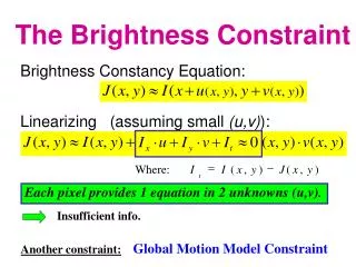
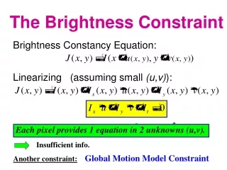
= - I I ( x , y ) J ( x , y ) Where: t Insufficient info. The Brightness Constraint Brightness Constancy Equation: Linearizing (assuming small (u,v)): Each pixel provides 1 equation in 2 unknowns (u,v). Another constraint:Global Motion Model Constraint
The 2D/3D Dichotomy Requires prior model selection 3D Camera motion + 3D Scene structure + Independent motions Camera induced motion + = Independent motions Image motion = 2D techniques 3D techniques Do not model“3D scenes” Singularities in “2D scenes”
The 2D/3D Dichotomy In the uncalibrated case (unknown calibration matrix K) Cannot recover 3D rotation or Plane parameters either (cannot tell the difference between a planar H and KR) The only part with 3D depth information When cannot recover any 3D info? • Planar scene:
* 2D models always provide dense correspondences. * 2D Models are easier to estimate than 3D models (much fewer unknowns numerically more stable). Global Motion Models Relevant for: *Airborne video (distant scene) * Remote Surveillance (distant scene) * Camera on tripod (pure Zoom/Rotation) 2D Models: • 2D Similarity • 2D Affine • Homography (2D projective transformation) 3D Models: • 3D Rotation + 3D Translation + Depth • Essential/Fundamental Matrix • Plane+Parallax Relevant when camera is translating, scene is near, and non-planar.
Least Square Minimization (over all pixels): Example: Affine Motion Substituting into the B.C. Equation: Each pixel provides 1 linear constraint in 6 global unknowns (minimum 6 pixels necessary) Every pixel contributes Confidence-weighted regression
Example: Affine Motion Differentiating w.r.t. a1 , …, a6 and equating to zero 6 linear equations in 6 unknowns: Summation is over all the pixels in the image!
Coarse-to-Fine Estimation Jw refine warp + u=1.25 pixels u=2.5 pixels ==> small u and v ... u=5 pixels u=10 pixels image J image J image I image I Pyramid of image J Pyramid of image I Parameter propagation:
Other 2D Motion Models 2D Projective – planar motion (Homography H)
Generated Mosaic image Panoramic Mosaic Image Original video clip Alignment accuracy (between a pair of frames): error < 0.1 pixel
Video Removal Original Original Outliers Synthesized
Video Enhancement ORIGINAL ENHANCED
Direct Methods: Methods for motion and/or shape estimation, which recover the unknown parameters directly from image intensities. Error measure based on dense image quantities(Confidence-weighted regression; Exploits all available information) Feature-based Methods:Methods for motion and/or shape estimation based onfeature matches (e.g., SIFT, HOG). Error measure based on sparse distinct features(Features matches + RANSAC + Parameter estimation)
Benefits of Direct Methods • High subpixel accuracy. • Simultaneously estimate matches + transformation Do not need distinct features for image alignment: • Strong locking property.
Limitations of Direct Methods • Limited search range (up to ~10% of the image size). • Brightness constancy assumption.
DEMO: Video Indexing and Editing • Exercise 4: Image alignment • (will be posted in a few days) • Keep reference image the same (i.e., unwarp target image) • Estimate derivatives only once per pyramid level. • Avoid repeated warping of the target image • Compose transformations and unwarp target image only.
Source of dichotomy: Camera-centric models (R,T,Z) Camera motion + Scene structure + Independent motions The 2D/3D Dichotomy Camera induced motion = + Independent motions = Image motion = 2D techniques 3D techniques Do not model “3D scenes” Singularities in “2D scenes”
The residual parallax lies on aradial (epipolar) field: epipole Move from CAMERA-centric to a SCENE-centric model Original Sequence Plane-Stabilized Sequence The Plane+Parallax Decomposition
1. Reduces the search space: • Eliminates effects of rotation • Eliminates changes in camera calibration parameters / zoom Benefits of the P+P Decomposition • Camera parameters: Need to estimate only the epipole. (i.e., 2 unknowns) • Image displacements: Constrained to lie on radial lines (i.e., reduces to a 1D search problem) A result of aligning an existing structure in the image.
2. Scene-Centered Representation: Benefits of the P+P Decomposition Translation or pure rotation ??? Focus on relevant portion of info Remove global component which dilutes information !
2. Scene-Centered Representation: Shape =Fluctuations relative to a planar surface in the scene Benefits of the P+P Decomposition STAB_RUG SEQ
total distance [97..103] camera center scene global (100) component local [-3..+3] component 2. Scene-Centered Representation: Shape =Fluctuations relative to a planar surface in the scene Benefits of the P+P Decomposition • Height vs. Depth (e.g., obstacle avoidance) • Appropriate units for shape • A compact representation - fewer bits, progressive encoding
3. Stratified 2D-3D Representation: • Start with 2D estimation (homography). Benefits of the P+P Decomposition • 3D info builds on top of 2D info. Avoids a-priori model selection.
Dense 3D Reconstruction(Plane+Parallax) Original sequence Plane-aligned sequence Recovered shape
Dense 3D Reconstruction(Plane+Parallax) Original sequence Plane-aligned sequence Recovered shape
Dense 3D Reconstruction(Plane+Parallax) Original sequence Plane-aligned sequence Recovered shape
p Epipolar line epipole Brightness Constancy constraint 1. Eliminating Aperture Problem P+P Correspondence Estimation The intersection of the two line constraints uniquely defines the displacement.
other epipolar line p Epipolar line another epipole epipole Brightness Constancy constraint 1. Eliminating Aperture Problem Multi-Frame vs. 2-Frame Estimation The other epipole resolves the ambiguity ! The two line constraints are parallel ==> do NOT intersect