Download
1 / 21
210 likes | 387 Vues
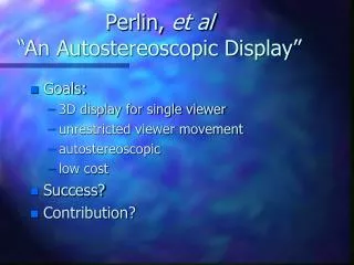
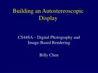
Building an Autostereoscopic Display. CS448A – Digital Photography and Image-Based Rendering Billy Chen. Original Goals. dynamic, real-time display convenient 3D display for the home (3D desktops) autostereoscopic light field viewer. Display design choices. Physical Setup. Render.

E N D
Building an Autostereoscopic Display CS448A – Digital Photography and Image-Based Rendering Billy Chen
Original Goals • dynamic, real-time display • convenient 3D display for the home (3D desktops) • autostereoscopic light field viewer
Render Overview of display process Calibration `
Calibration • affine transformation correction (mostly scale) • projective transformation correction
Calibration solution 1 • OpenGL program displays a moiré pattern • can calibrate up to affine transformations • most effective for finding correct size
Calibration solution 2 p A’ A h p B B’ Finding the homography without getting projector parameters
Calibration solution 2 x y 1 cx’ cy’ c M = M p cp’ Let Mi = i’th row of M (1) M1p = cx’ (2) M2p = cy’ (3) M3p = c y’ (M1p) - x’(M2p) = 0 M1p - x’(M3p) = 0 M11 xy’ yy’ y’ -xx’ -yx’ -x’ 0 0 0 M12 = 0 M13 . . M21 . . . . 9x1 8x9 A= Take SVD(A) and look at matrix
Rendering • sampling the light field • computing lenslet distances • cropping and compositing
Rendering: Sampling a light field Isaksen et al., Siggraph 2000
Getting “floating” images Halle, Kropp. SPIE ‘97
Rendering: compositing and cropping images crop subsample composite
Implementation Details • Fresnel hex array #300; 0.12 in. focal length, 0.12 in. thickness, .09 in. diameter • default size for a lenslet image: 26x31 pixels (for 300 dpi displays) • calibrate scale is .49 (sanity check: 300 dpi / 150 dpi) • OpenGL unit == 1 pixel (300 dpi) • SEE WEBPAGE!
Results compared to original goals • real-time display is hard, must handle the bandwidth • spatial resolution too small for 3D desktops • light fields have problems with much depth complexity, but NEED depth for effective autostereoscopic displays
Future Work • reflective display • auto-calibration • hardware accelerated light field sampling • overloading pixels per direction: perspective views, displacing display pixels from focal plane • use a light field of captured data
Acknowledgements • calibration: Vaibhav Vaish • light field generator: Georg Petschnigg • hardware accelerated approach: Ren Ng • bootstrap: Sean Anderson