Download

1 / 15
150 likes | 372 Vues
ATOP Nowcast & Forecast – an Example. Today’s Date (TDD=2012-03-10) & Time of Nowcast (i.e. Analysis) & Forecast: TDD /10AM Forecast GFS Wind is Available at: TDD /8~9:30AM (/archive/hunglu/Oceanus/cron_gfs_download_interp/out/gfsw_20120317.nc)

E N D
ATOP Nowcast & Forecast – an Example Today’s Date (TDD=2012-03-10) & Time of Nowcast (i.e. Analysis) & Forecast: TDD/10AM Forecast GFS Wind is Available at: TDD/8~9:30AM (/archive/hunglu/Oceanus/cron_gfs_download_interp/out/gfsw_20120317.nc) AVISO Data is Available from Previous Day: TDD-1d (e.g. 2012-03-09 for TDD= 2012-03-10) (/archive/lameixisi/AVISO/for_netcdf/nc2sbpom/out/msla_20120309.nc) 14 Days: Nowcast & Forecast Dates: From TDD-7d TDD TDD TDD+7d i.e. 2012-03-03 2012-03-10 (nowcast) 2012-03-10 2012-03-17 (forecast) Outputs in /archive/lyo/mpiPOM/pac10/exp302/out restart.2012-03-04_00_00_00.nc for next-day’s (i.e. for 2012-03-11) forecast SRF.pac10exp302.2012-03-03_to_2012-03-17.nc Daily surface fields pac10exp302.2012-03-03_to_2012-03-17.nc 2 x 7day-averaged 3-D fields Plots: Whole Pacific (e.g. msla_SSH-SSHA_20120308.ps) Fig.1a (top panel): Model SSH field on the 7th day (i.e. TDD=2012-03-10); Fig.1b (mid panel): AVISO SSH field on the same day (or closest to the same day); Fig. 1c (bot panel): Colors of RMS(η’M-η’A) computed over moving 5ox5o (or ~50x50 pac10 grids), then superimpose contours of Correlate(η'M,η'A) also over the moving 5ox5o; where η' = η - <η> & <η> = 5ox5o smoothed field of η Fig. 2 – same as Fig.1 but for SSHA . For model SSHA = SSH – ELAV from binary correlation FORTRAN output. Note that in this case, for Fig.2c, since we already have the anomaly (η‘), it is not necessary to define < η>. SCS Domain (e.g. msla_SSH-SSHA_SCS_20120308.ps) Fig. 3a,b,c,d (4 panels on 1 page): Daily color SSH with surface (u,v) as trajectories, day 7, 8, 9 & 10 Fig. 4a,b,c,d (4 panels on 1 page): Daily color SSH with surface (u,v) as trajectories, day11,12,13 & 14 Runscript: /wrk/lyo/mpiPOM/pac10/exp302/ batch_run_profs-fcast.csh
Routine Tasks Yoyo, I would like you to make plots of downloaded data each time: 1. Satellite data SSH & SSHA plots – page 1 is for the entire pac10 domain: top panel is SSH & bottom panel is ssha; page 2 is western North Pacific west of 140E and from -10S to 40N; 2. Same as “1” but for the wind data. I also would like you to describe and report these plots to me on our Friday progress meeting – as part of your presentation. Thank you. Leo
Yoyo’s pac10-analysis tasks, A & B pac10-analysis locations B. Compare in details with Taiwan ship-ADCP Data: seasonal means. A. Compare in details with satellite in Luzon Strait & South China Sea: 1. means & StdDs: xy-contours (maps) both SSHA & geostrophic currents (mean+variance ellipses); 2. seasonal I hope you can present these results for your PhD Entrance exam to NCU in May/2012
pac10-analysis: transects A-G G. Tsushima Strait transport D. Transport through the Taiwan Strait – mean & seasonal: ship ADCP H. JMA-Section (137oE,3-34oN) E. Kuroshio Transport at PN-line, mean & seasonal B. Compare in details with ADCP’s: means & StdDs: 1. xz-contours; 2. Transport time-ser + mean & StdD; Johns, W.E., T.N. Lee, D. Zhang and R. Zantopp, 2001: The Kuroshio east of Taiwan: moored transport observations from the WOCE PCM-1 array. J.Phys.Oceanogr., 31, 1031–1053. C. Flows across the Luzon Strait – upper & lower & whole, mean & seasonal A. Kuroshio Transport off Luzon at ~18N, mean & seasonal – see Sheu, Wu & Oey (2010) F. Karimatan Strait: transport
Alu’s pac10-analysis STCC pac10-STCC analysis Means, eddies + PV etc: is there an STCC in the model? Alu, you have read many papers – so now you can apply what you have learned. BTW, I still want you to finish up your idealized case – do that first for OSM!! Write a DRAFT paper based on what you have.
pac10-analysis: transects A-G G. Tsushima Strait transport D. Transport through the Taiwan Strait – mean & seasonal: ship ADCP E. Kuroshio Transport at PN-line, mean & seasonal B. Compare in details with ADCP’s: means & StdDs: 1. xz-contours; 2. Transport time-ser + mean & StdD; Johns, W.E., T.N. Lee, D. Zhang and R. Zantopp, 2001: The Kuroshio east of Taiwan: moored transport observations from the WOCE PCM-1 array. J.Phys.Oceanogr., 31, 1031–1053. C. Flows across the Luzon Strait – upper & lower & whole, mean & seasonal A. Kuroshio Transport off Luzon at ~18N, mean & seasonal – see Sheu, Wu & Oey (2010) F. Karimatan Strait: transport
IHOS - Taiwan Ocean Prediction (TOP) Research Highlights; Oct/20/2011; by L.Oey. • IHOS is developing an ocean current and wave prediction model: the Taiwan Ocean Prediction (TOP) system that eventually will include also air-sea (with typhoons) and air-sea-ice coupling, as well as biogeochemical processes. Three recent publications and an example of the simulated SST over the entire North Pacific Ocean are given below. • Chang, Y.-L. & L.-Y. Oey, 2011: The Philippines-Taiwan Oscillation: Monsoon-Like Interannual Oscillation of the Subtropical-Tropical Western North Pacific Wind System and Its Impact on the Ocean. J. Climate, in press. PDF Format. Download PTO Data (text file) here. • Chang, Y.-L., and L.-Y. Oey, 2011: Interannual and seasonal variations of Kuroshio transport east of Taiwan inferred from 29 years of tide-gauge data, Geophys. Res. Lett., 38, L08603, doi:10.1029/2011GL047062 • Fujisaki, A. and L.‐Y. Oey, 2011: Formation of ice bands by winds, J. Geophys. Res., 116, C10015, doi:10.1029/2010JC006655. TOP sea-surface temperature (SST) on Jun/06/1988 during the developing stage of the strong 88-89 La Niña when waters as cold as 19oC is simulated in the eastern equatorial Pacific in excellent agreement with observation (http://www.pmel.noaa.gov/tao/elnino/la-nina-story.html#). TOP also simulates a beautiful meandering Kuroshio that separates off the eastern coast of Japan, as well as the intrusion of very warm waters (SST≈31oC) into the South China Sea through the Luzon Strait. (From Lu, H.-F. & L.-Y. Oey, 2011: Instability waves and eddies of the Subtropical Counter Current in the North Pacific Ocean, Manuscript in preparation).
pac10-analysis locations B. Compare in details with Taiwan ship-ADCP Data: seasonal means. C. Compare in details with ADCP’s: means & StdDs: 1. xz-contours; 2. Transport time-ser + mean & StdD; Johns, W.E., T.N. Lee, D. Zhang and R. Zantopp, 2001: The Kuroshio east of Taiwan: moored transport observations from the WOCE PCM-1 array. J.Phys.Oceanogr., 31, 1031–1053. A. Compare in details with satellite in Luzon Strait & South China Sea: 1. means & StdDs: xy-contours (maps) both SSHA & geostrophic currents (mean+variance ellipses); 2. seasonal